eyeprolog
This book is licensed under Creative Commons Attribution 4.0 International. You may copy, share, and adapt it for any purpose, including commercially; please give appropriate credit, link to the licence, and indicate changes.
EyeProlog turns facts and rules into answers and inspectable proofs. This book is an original introduction to the habits of logic programming: describe a world, state the relationships that hold in it, and let unification and search connect the two.
This book is also the reference for the EyeProlog implementation. EyeProlog is a standards-based reasoning system: programs use the documented and tested ISO Prolog profile. Chapters 38–40 define the supported ISO Prolog profile, predicate surface, libraries, and execution interface. Chapter 39 describes every supported built-in and library predicate, with compact contracts for all 533 distinct predicate indicators in the normal EyeProlog surface; Chapter 40 documents command-line execution. The explanatory chapters give the reasoning and operational context needed to use those details correctly.
Its subject is not syntax alone. A logic program has two inseparable aspects: the relation described by its clauses and the procedure induced when goals are selected and clauses are tried. The first tells us what answers are justified; the second tells us whether and how the machine will find them. Learning to program with EyeProlog means learning to move comfortably between these views.
EyeProlog implements a broad ISO Prolog profile with facts, clauses, terms, lists, control, arithmetic, dynamic predicates, operators, streams, and standard built-ins. Explicit tabling, explicit integrity checks, and proof output are implementation capabilities around that standards-based foundation. EyeProlog does not claim formal certification against every ISO processor edge case.
Standards are crucial because knowledge and rules often outlive the software that first processes them. Using ISO Prolog keeps programs teachable, inspectable, and portable across processors. EyeProlog aims to provide a compact implementation of that standard with explanations and practical host integration, not another proprietary rule language.
This places EyeProlog in a tradition that joins automated deduction, database querying, and programming. Jacques Herbrand’s doctoral work made ground terms and ground instances central to proof theory; Robinson’s later resolution principle turned unification and refutation into a general proof procedure; early Prolog showed that Horn clauses could also be executable programs; deductive databases emphasized finite relations and fixed points. EyeProlog borrows from all three traditions without pretending that they are identical. Its clauses are logical statements, its query execution is an ordered computation, and its proof terms make the connection between the two available for inspection.
That history explains a recurring theme of the book. Logic programming is not the claim that control disappears. It is the discipline of stating the relation clearly enough that control can be studied and improved separately. Robert Kowalski’s phrase “algorithm = logic + control” names this separation; EyeProlog’s focused surface makes it unusually easy to see in running examples.
Complete EyeProlog code displays from the book are also available as files under
examples/book/, grouped by chapter. From a source checkout
with Node.js 18 or newer, run the CLI directly:
node bin/eyeprolog.js examples/socrates.pl
The EyeProlog command should print:
type(socrates, mortal).
holds_result(test, true).
A run answers in Prolog: each goal a query proved, with that answer’s bindings applied. The output is an ordinary program, so it can be saved, loaded and queried like any other.
Then ask for the derivations:
node bin/eyeprolog.js --proof examples/socrates.pl
To use the published package, first verify that node --version reports Node.js
18 or newer. Upgrade an older runtime through a Node version manager or the
official Node.js download. A current Linux
distribution can still expose an older Node.js package.
The package can be launched without a global installation:
npx --yes eyeprolog
For a persistent command without administrator access, install into a user-owned prefix:
npm install --global --prefix "$HOME/.local" eyeprolog
export PATH="$HOME/.local/bin:$PATH"
Persist the PATH export in the appropriate shell startup file. Do not use
sudo npm install; npm’s
EACCES guidance
recommends a Node version manager or a user-owned npm prefix.
Readers who do not want to install anything can begin in the
browser playground. Paste
the source of examples/socrates.pl into the editor and run it. The playground
and local CLI accept the same in-memory Prolog source and resolve the same
standard modules. A program imports relations such as append/3 and member/2
with use_module(library(lists)). The page starts src/playground-worker.js as
a dedicated ES-module worker for each run. Serve a
local checkout over HTTP(S), rather than opening the page as a file: URL.
Filesystem predicates and include/1 are Node-only; URL and embedding examples
require their documented host environment.
The best way to read is beside a running interpreter. Before each run, predict the answer; after it, change one fact or query and explain the difference.
Reading conventions
Code displays serve three different purposes:
- an
eyeprologblock is Prolog source accepted by EyeProlog; complete blocks also appear underexamples/book/, although a short block may rely on facts introduced in the surrounding chapter; - a
textblock shows output, a trace, a data shape, or pseudocode and is not necessarily accepted as EyeProlog input; - a
shorjsblock is a host command or embedding example.
Top-level programs under examples/ are the complete runnable
cases. Their exact outputs live under examples/output/, the proof of each
under examples/proof/, and the result of checking that proof under
examples/check/. Use examples/book/ to copy a particular display and the
top-level corpus for end-to-end experiments.
The promise of this book
This book treats logic programming as a craft, not a collection of clever tricks. By the end, a reader should be able to:
- state a domain as relations whose ground instances have an unambiguous meaning;
- read every clause both as a logical sentence and as a computation;
- design finite searches, justify termination, and recognize when a calling mode is unsafe;
- construct programs from examples and invariants, then improve their control without quietly changing their meaning;
- test conclusions, detect inconsistent inputs explicitly, and inspect proofs as evidence; and
- connect a Prolog rule set to JavaScript without hiding the host boundary.
That is the stake in the ground: a focused implementation of standard Prolog is enough to teach the large ideas when semantics, execution, and evidence remain visible together. The implementation is therefore part of the argument: the examples are executable programs, the reference chapters describe the running system, and proof terms remain available for inspection.
A working discipline
Approach each example through the same six moves:
- Sentence. Say what one ground instance means.
- Question. Choose the bindings with which the relation will be called.
- Prediction. Write the expected answers before running the program.
- Search. Trace the first choice, the bindings it adds, and the next goal.
- Evidence. Inspect a proof and distinguish it from the failed search branches that were explored.
- Revision. Change one fact, query, goal order, or representation and explain what should remain invariant.
This rhythm deliberately joins declarative reading, operational reading, and program construction. Readers new to logic programming can follow Parts I–III in order. Experienced Prolog programmers can begin with Chapters 3, 13, and 17 to see how EyeProlog combines ordinary depth-first Prolog with explicit tabling, Eyelet forward rules, and inspectable proofs. Chapter 41 gives further routes through the material.
When a run surprises you
Do not change several clauses at once. Use this recovery loop:
- reduce the issue to the smallest ground question whose answer you dispute;
- confirm that every predicate in that question has one clear sentence;
- write the bindings available before each body goal from left to right;
- run with
--proofif an unexpected answer succeeds; - run with
--statsor hand-trace the first branch if an expected answer is missing or slow; - preserve the discovery as a test before repairing the program.
No output can mean a legitimate absence, suppression of a queried source fact, an unready built-in, or an unfinished search. Chapter 1 introduces source-fact suppression, Chapters 7 and 11 distinguish failure from printed output, and Chapter 32 develops the full debugging method.
Choose a route
The book supports several paths; reading every chapter in order is not a test of seriousness.
| Reader | Suggested route | What to postpone |
|---|---|---|
| New to programming | Chapters 1–10, 11–12, 18–20, then Laboratories 1–4 | The formal parts of Chapter 3, embedding, and Parts V–VI |
| Programmer new to logic | Parts I–II, Chapters 11–13 and 17–25, then Part VII | Detailed history and mathematical foundations on the first pass |
| Experienced Prolog programmer | Chapters 3, 7, 11–13, 16–17, and 31–33 | Introductory syntax and list material |
| Knowledge engineer | Chapters 7, 11–16, 25, 31–33, then Laboratories 9–12 | Symbolic mathematics unless it serves the domain |
| Mathematics reader | Chapters 1–5, 19, and 26–30 | Embedding until an application needs it |
| Instructor or study group | Parts I–III, one route through Part V or VI, then selected laboratories | Reference chapters until reference work begins |
On a first pass, treat sections marked Deeper foundations as optional. They make the semantics precise but are not prerequisites for writing and running the next program.
The construction order
The sequence follows the teaching architecture associated with The Art of Prolog: begin with the meaning of a relation, make the relation executable, study the control it induces, and then return to the same ideas at a larger scale through transformation, search, interpreters, and applications. Each part therefore ends by asking the reader to construct, test, or improve a program rather than merely recognize syntax. Reference material follows practice, laboratories turn the methods into work, and checkpoint notes close the loop with retrieval and diagnosis.
Balance here does not mean that every chapter has the same length or the same number of pictures. A language catalog should be searchable; a construction chapter should be argumentative; a laboratory should leave an artifact. The recurring balance is instead between four readings of a program:
| Reading | Question carried through the book | Typical evidence |
|---|---|---|
| Meaning | What does each ground relation claim? | a domain sentence and examples |
| Computation | How are answers actually found? | a trace, finite bound, or termination measure |
| Construction | Why is the program shaped this way? | a worked refinement and rejected alternative |
| Judgment | What has been established, and what remains assumed? | tests, proofs, counterexamples, and a trust boundary |
Diagrams follow the same rule. Scenes introduce an intuition; structural diagrams expose a term, proof, or dependency; process diagrams guide a piece of work; maps help navigate reference and review. A diagram earns its place by making a relationship visible that prose alone would make easy to miss.
Contents
Chapters are numbered continuously across eleven parts, from Chapter 1 to Chapter 45.
Part I — Relations
Chapters 1–5
- 1. A program is a little theory
- 2. Terms, variables, and substitution
- 3. Rules and their two readings
- 4. Recursion: describing reachability
- 5. Lists as relations
Part II — Search
Chapters 6–10
- 6. Arithmetic and finite generation
- 7. Failure, negation, and quantification
- 8. Collecting and choosing answers
- 9. Structured data, text, and contexts
- 10. From puzzles to models
Part III — Trustworthy reasoning
Chapters 11–16
- 11. Queries, answers, and proofs
- 12. Integrity checks as ordinary predicates
- 13. Termination, tabling, and performance
- 14. Knowledge engineering
- 15. Explicit data boundaries
- 16. Embedding EyeProlog
Part IV — The craft of logic programming
Chapters 17–20
- 17. Logic and control
- 18. Constructing a program
- 19. Correctness and termination
- 20. Improving a program
Part V — Advanced relational design
Chapters 21–25
- 21. Reading the computation
- 22. Trees, languages, and symbolic evaluation
- 23. Transforming programs
- 24. Designing finite search
- 25. Case study: an auditable decision service
Part VI — Mathematics made executable
Chapters 26–30
- 26. A proof can be a computation
- 27. Recursion is induction in motion
- 28. Algebra, symmetry, and representation
- 29. Search as experimental mathematics
- 30. What mathematics promises
Part VII — The reasoning laboratory
Chapters 31–33
- 31. Testing a theory
- 32. Debugging by meaning, search, and proof
- 33. A pattern catalog for reasoning
Part VIII — Standard Prolog in practice
Chapters 34–37
- 34. Control, exceptions, and grouped solutions
- 35. Reflective terms and atomic conversion
- 36. Dynamic predicates, directives, and operators
- 37. Streams and term I/O
Part IX — Reference as practice
Chapters 38–43
- 38. Language and ISO profile
- 39. Predicate reference
- 40. Running EyeProlog: command line and corpus
- 41. Study paths, review, and further examples
- 42. Standards, limits, and implementation boundaries
- 43. Glossary and notes for continued study
Part X — Laboratories
Chapter 44
Part XI — Review
Chapter 45
Part I — Relations
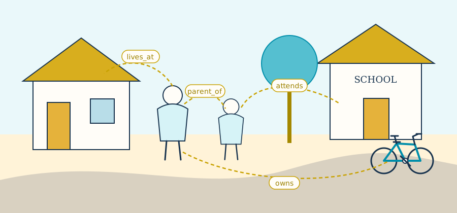
We begin with connection rather than calculation. Facts place points in a relational world; variables draw threads between them; rules make one pattern follow from another.
1. A program is a little theory
Logic programming begins with a change of emphasis. Instead of listing the steps that calculate an answer, write sentences that are true in the problem domain.
parent(ada, byron).
parent(byron, clara).
parent(clara, diego).
Each line is a fact. parent/2 is a relation: the name is parent and the
arity is two. Arity matters. parent/2 and parent/3 are different predicates.
A host-supplied query selects the relation whose ground answers EyeProlog prints:
child(Child, Parent) :- parent(Parent, Child).
eyeprolog --goal 'child(X, Y)' program.pl
The answers are:
child(byron, ada).
child(clara, byron).
child(diego, clara).
EyeProlog distinguishes solutions found by the solver from answers printed by the
CLI. A query such as eyeprolog --goal 'parent(X, Y)' program.pl can find the three source facts
internally, but the normal CLI output suppresses answers that merely repeat
source facts. Derived child/2 answers are printed. Chapter 11 explains this
output policy; it does not change what calls inside rules can prove.
The program did not copy values through named slots. It found substitutions
for Child and Parent that made the rule body true, then applied those same
substitutions to the head.
Before writing a relation, ask:
- What does one ground fact mean as a sentence?
- Which arguments are normally known when it is called?
- Is the relation finite in that calling pattern?
For parent(Parent, Child), a ground fact reads naturally from left to right.
Calling it with a parent enumerates children; calling it with a child enumerates
parents; calling it open enumerates the finite database. A good relation has a
clear sentence and useful modes.
Facts are data, not commands. Clause order can affect search order, but a fact does not mean “do this now.”
Learning to see relations
The shift from functions to relations takes practice. A function is normally introduced with a direction: put an input in one side and receive an output from the other. A relation begins with a set of tuples. Direction enters only when somebody asks a question.
Take parent/2. The program does not store a procedure named “find children.”
It stores pairs for which the relation holds. From that single relation, one
may ask for a child’s parents, a parent’s children, whether two named people
stand in the relation, or every known pair. The source text stays fixed while
the binding pattern changes.
This is why the wording of a predicate matters. Before adding a rule, read a ground instance aloud:
parent(ada, byron)means that Ada is a parent of Byron.
Now replace one name at a time with a question:
For which
Childis Ada a parent?Who is a
Parentof Byron?Which
Parent–Childpairs are known?
If those questions feel like natural uses of one statement, the relation is probably well shaped. If each reading requires a different interpretation of an argument, split the concept before the ambiguity spreads into later rules.
Exercise. Add grandparent/2 using two calls to parent/2. Query all
grandparents, then only the grandparents of diego.
Checkpoint. Before continuing, make sure you can (1) read
parent(ada, byron) as a sentence, (2) explain what the two variables in
eyeprolog --goal 'child(X, Y)' program.pl ask for, and (3) predict which output changes after adding
parent(diego, elena).
2. Terms, variables, and substitution
Prolog programs accepted by EyeProlog are built from terms:
- atom constants:
ada,accepted,'atom with spaces'; - double-quoted character lists:
"sensor too hot"(the default shorthand for[s,e,n,s,o,r,' ',t,o,o,' ',h,o,t]); - numbers:
42,-7,3.14159,1.2e3; - variables:
X,Person,_temporary; - compound terms:
point(3, 4),reading(temp, 91); - lists:
[],[red, green, blue],[Head | Tail].
In normal mode, double-quoted character/code lists also support Trealla’s
right-splice notation. With double_quotes(chars), "ab"||Tail is shorthand
for [a,b|Tail]; with double_quotes(codes), it denotes [97,98|Tail]. The
splice is not available when double_quotes(atom) is active, and
--iso-strict rejects it as an implementation-specific syntax extension.
Normal-mode integer constants may use one underscore between adjacent digits,
as in 1_000 or 0xCA_FE. Layout, including comments and newlines, may follow
the underscore before the next digit. Separators do not apply to floating-point
fractions or exponents, and --iso-strict rejects them.
Plain atom constants begin with a lowercase ASCII letter. Variables begin with
an uppercase letter or underscore. The bare _ is anonymous and every
occurrence is fresh. _Name is a named variable; repeated occurrences refer to
the same variable within its clause. Variables are local to a clause.
Unification
Unification asks whether two terms can be made identical by binding variables.
reading(Sensor, 91)
reading(temp, Value)
They unify with Sensor = temp and Value = 91. Structure must agree
recursively. point(X, X) unifies with point(2, 2) but not point(2, 3).
Functor and arity must agree.
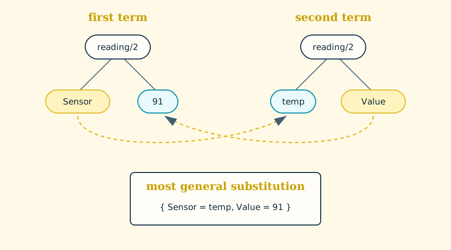
The picture is worth lingering over. Unification does not assign values in a one-way parameter list. It aligns two structures. A variable on either side may receive a binding; a nested pair of compounds causes the same comparison to continue recursively. The result shown is the most general substitution: it commits to exactly what structural agreement requires and nothing more.
EyeProlog exposes unification as =/2:
same_shape(Pair) :- (Pair = pair(X, X)).
eyeprolog --goal 'same_shape(pair(red, red))' program.pl
eyeprolog --goal 'same_shape(pair(red, blue))' program.pl
Only the first query succeeds. \=/2 succeeds when two resolved terms are not
structurally equal.
Compound terms retain domain structure:
:- use_module(library(lists)).

measurement(battery_1, sample(17, volts(28.4), amps(12.1))).
route(a, d, path([a, b, d], cost(9))).
As a fact head, measurement(...) is an atomic formula. Nested terms are data.
The same surface form serves both roles; context decides which.
ready is an atom constant and "ready" is, by default, a proper list of
one-character atoms. Keep symbolic vocabulary as atoms and use character lists
when text must be inspected relationally. Quoted atoms remain atoms:
label(sensor_1, "Cabin temperature").
web_name(sensor_1, '<https://example.org/sensor/1>').
Exercise. Write diagonal/1, which succeeds for point(X, X). Then write
same_ends/1 for a three-element list whose first and last values agree.
Checkpoint. Without running EyeProlog, decide whether each pair unifies:
point(X, X) with point(red, red), point(X, X) with
point(red, blue), and [Head | Tail] with [a, b, c]. Then run a small
=/2 query to check each prediction.
3. Rules and their two readings
The executable-clause idea emerged from work on automated theorem proving. Robinson’s resolution principle supplied a general proof rule, while the development of Prolog specialized proof search around clauses that could be read as procedures. EyeProlog begins further downstream: it offers a compact definite-clause language rather than a general first-order theorem prover. The restriction buys a direct correspondence between a rule body and the subquestions used to establish its head.
A rule has a head and a comma-separated body:
:- use_module(library(lists)).

eligible(Person) :-
  age(Person, Years),
  (Years >= 18),
  registered(Person).
Read it declaratively: a person is eligible if the person has an age of at least 18 and is registered. Read it operationally: to solve the head, solve the body goals in their written dependency order, carrying bindings into later goals. EyeProlog normally selects from left to right. As a safe optimization, it may run a ready deterministic built-in filter early; such a filter cannot add alternative answers and already has the inputs its registered mode requires.
Both readings matter. The declarative reading checks the model. The operational reading helps make search finite and selective. Put a generator before a built-in that needs its input.
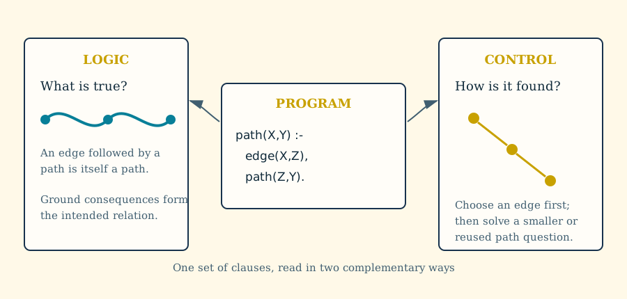
The two readings are not rivals. The logical reading prevents an efficient program from quietly answering the wrong question. The operational reading prevents a beautiful specification from wandering forever without producing an answer. Much of the craft in this book consists of keeping one reading steady while improving the other.
:- use_module(library(lists)).

adult(Person) :-
  age(Person, Years),
  (Years >= 18).
Multiple clauses express alternatives:
can_enter(Person) :- staff(Person).
can_enter(Person) :- visitor(Person), escorted(Person).
Helper predicates reveal the model and improve explanations:
high_score(Case) :-
  score(Case, Score),
  threshold(Threshold),
  (Score >= Threshold).

status(Case, accepted) :- high_score(Case).
reason(Case, "score meets threshold") :- high_score(Case).
Deeper foundations: Herbrand’s move
This section through “Meaning is not the search strategy” supplies the formal model behind the earlier examples. On a first practical reading, it is safe to continue at Chapter 4 and return here after writing a recursive relation.
The terminology in the next section honors a remarkably early source. Jacques Herbrand developed the relevant ideas in his 1930 doctoral thesis, Recherches sur la théorie de la démonstration (“Investigations in proof theory”). His fundamental theorem connected first-order derivability with propositional reasoning over suitably chosen ground instances. In broad terms, quantified proof obligations could be studied through formulas obtained by substituting constructed terms for variables.
That move supplied more than names. It made syntax usable as a mathematical universe: constants and function symbols generate ground terms, and atomic formulas over those terms provide a concrete space in which proofs can be analyzed. This viewpoint became foundational for automated theorem proving. Unification can be understood as finding substitutions that bring symbolic formulas together, while later proof procedures can search among clause instances without first assigning terms to an unrelated external domain.
The historical distinctions matter. Herbrand did not invent Robinson’s 1965 resolution calculus, nor did his thesis state the later least-model semantics of logic programs in its modern form. Rather, his proof theory laid essential groundwork. Resolution supplied a powerful subsequent inference mechanism, and van Emden and Kowalski later gave definite logic programs their fixed-point and least-Herbrand-model account. EyeProlog sits downstream of this sequence:
Herbrand: ground terms and instances as a proof-theoretic foundation
  -> Robinson: resolution and unification as a proof procedure
  -> logic programming: executable clauses and least-model semantics
  -> EyeProlog: a focused Prolog implementation with inspectable derivations
Herbrand completed this work while still in his early twenties and died in
- The scale of its later influence—in proof theory, automated deduction, and logic programming—is one reason the word Herbrand recurs throughout this book rather than appearing only as historical attribution.
The Herbrand world
The declarative reading needs a precise answer to a deceptively simple question: what can a term denote? EyeProlog uses Herbrand semantics. Its universe contains exactly the ground terms that can be constructed from the program’s atom constants, numbers, list constructors, and compound functors. There are no unnamed elements hiding behind the notation. A ground term denotes itself.
This separates the Herbrand universe, whose members are terms such as
pat, 3, [red, blue], and ticket(alice), from the Herbrand base,
whose members are ground atomic formulas such as person(pat) and
owns(alice, ticket(17)). A term is not true or false merely by existing:
pat is a possible argument, whereas person(pat) is a proposition that an
interpretation may make true.
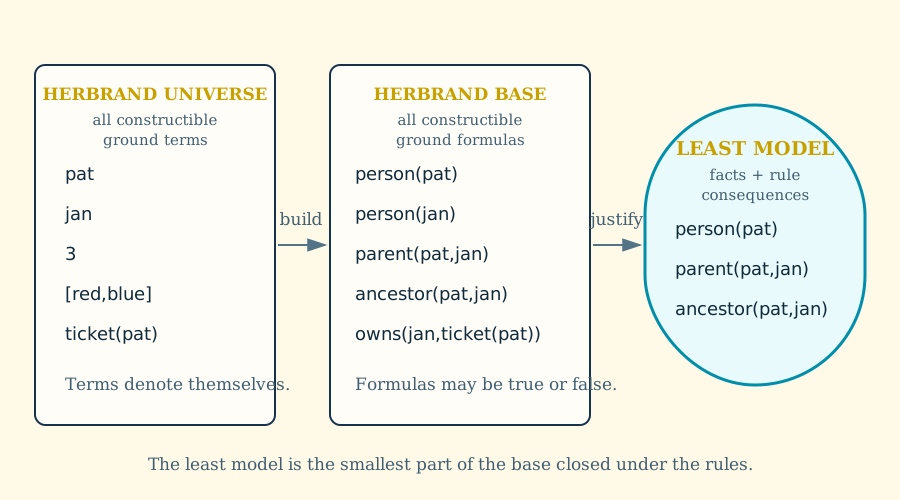
This three-level distinction answers several recurring questions. A newly constructed term does not automatically assert anything. A formula that can be written is not automatically true. And the model is not an arbitrary collection of convenient formulas: it is the smallest collection forced by the program. Keeping those levels separate makes symbolic data safe to inspect without confusing mention with assertion.
A Herbrand interpretation is a set of ground atomic formulas regarded as true. A source fact contributes one such formula:
parent(pat, jan).
A rule stands for all of its ground instances. Thus:
ancestor(X, Z) :- parent(X, Y), ancestor(Y, Z).
says that for every substitution of X, Y, and Z by Herbrand terms, truth
of both body formulas entails truth of the head formula. Variables in rules
are implicitly universally quantified.
The declarative meaning of a pure Prolog program is its least Herbrand model: the smallest interpretation containing every fact and closed under every rule. One mathematical way to obtain it is the immediate-consequence operation. Begin with the facts; add each ground rule head whose ground body is already true; repeat until reaching the least fixed point. This construction defines meaning. It does not prescribe that the implementation enumerate the model from the bottom up.
Why terms denote themselves
Herbrand semantics is a particular form of ordinary model theory, chosen because logic programs inspect and construct symbolic terms. Consider:
different(alice, bob) :- (alice \= bob).
different(ticket(alice), ticket(bob)) :-
  (ticket(alice) \= ticket(bob)).
In an unrestricted first-order interpretation, alice and bob could denote
the same object unless a unique-name axiom forbids it. Even if they denote
different objects, the interpretation of ticket need not be injective.
Additional axioms would be required to show that ticket(alice) and
ticket(bob) differ.
In the Herbrand universe those terms differ by construction. Different atom
constants are different terms; compound terms are free constructors and are
identical only when functor, arity, and corresponding arguments are identical.
Lists follow the same rule through [] and the internal ./2 constructor.
Unification, read-back, witness construction, and proof explanations therefore
share one predictable notion of identity.
This is a property of the representation, not a claim that two names can never
refer to one real-world entity. If robert and bob name the same person, say
so with same_as(robert, bob) or normalize them to one canonical term. The
Herbrand layer keeps names unambiguous; domain rules express equivalence.
The runnable
examples/herbrand-semantics.pl example and
its normal and proof outputs make this distinction concrete.
Quantification and visible witnesses
Variables range over Herbrand terms, not external records, pointers, or host-language objects. Variables in a selected goal are existential in the logic-programming sense: EyeProlog searches for substitutions that make the goal follow from the program.
EyeProlog has no blank nodes or existential variables in rule heads. When a rule needs to name a consequent object, construct an explicit witness:
has_parent(Child, parent_of(Child)) :-
  person(Child).

registration(Student, Course, registration_of(Student, Course)) :-
  takes(Student, Course).
The same inputs construct the same witness term; different inputs construct different terms. The witness is printable, queryable, and visible in a proof, rather than being an anonymous object created behind the program’s back.
Equality, unification, and the occurs check
Equality in the pure Herbrand reading is syntactic identity after substitution. Operationally, unification discovers a substitution that makes terms identical. EyeProlog performs an occurs check whenever unification would bind a variable. It therefore uses finite-tree unification and rejects a binding when the variable occurs anywhere in the proposed value. For example, the body of this clause fails rather than constructing a cyclic term:
cyclic_unification :- X = wrapper(X).
The goal has to be written inside a clause of its own: ISO 7.4.3 forbids a
Prolog text from supplying clauses for a built-in predicate, so a bare
(X = wrapper(X)). in a program file is a clause for (=)/2 and is rejected
with permission_error(modify, static_procedure, (=)/2).
ISO classifies unifications whose outcome depends on an occurs check as
subject-to-occurs-check (STO). EyeProlog’s default remains the sound finite-tree
behavior above. For diagnosis, EyeProlog additionally provides the
implementation-specific flag occurs_check; setting it to error turns a
normal unification that would otherwise fail because of the occurs check into
a representation error:
:- set_prolog_flag(occurs_check, error).

sto_example :- X = wrapper(X).
% error(representation_error(term), [])
The ISO error mechanism wraps an error term together with an
implementation-defined context term. For this implementation-specific STO
diagnostic EyeProlog uses representation_error(term) and currently uses the
empty list [] as that context. This reports that the cyclic result of a
succeeding STO unification cannot be represented by EyeProlog’s finite-tree
term model, without exposing a non-standard occurs_check/2 error term.
The supported values are true (the default finite-tree behavior) and error
(STO detection). EyeProlog deliberately does not provide occurs_check=false,
because its term model does not construct cyclic terms. The ISO predicate
unify_with_occurs_check/2 is independent of the diagnostic flag: it continues
to perform finite-tree unification and fails on unify_with_occurs_check(X,
wrapper(X)) even when occurs_check is error.
Meaning is not the search strategy
EyeProlog’s evaluator is goal-directed. It resolves selected goals against facts, rules, and built-ins using ordered conjunction, clause selection, indexing, tabling, and deterministic host operations. Written order defines the normal dataflow; a mode-ready deterministic built-in may be selected early as a pure filter. For the pure Horn-clause fragment, the answers it finds are intended to belong to the least Herbrand model. The evaluator is not, however, a complete bottom-up enumerator. Infinite generation or nonterminating recursion can prevent it from reaching a true answer.
Built-ins extend the pure core. Relational built-ins such as =/2,
append/3, and member/2 are readily understood over Herbrand terms.
Arithmetic, date handling, regular expressions, aggregation, once/1, and
negation have additional operational definitions. They still consume and
produce Prolog terms: X is 2 + 3 binds X to the Herbrand number term 5,
not to an invisible host value.
\+ Goal succeeds when the current finite search finds no solution for
Goal; it does not insert a negative formula into the Herbrand model.
User-defined negative dependencies should be stratified. In a stratified
program, positive dependencies may remain in the same or a lower layer, while
every negative dependency points strictly downward:
closed(X) :- blocked(X).
open(X) :- candidate(X), \+ closed(X).
A cycle containing a negative edge is not stratified:
p(X) :- q(X).
q(X) :- \+ p(X).
The CLI reports such portability problems with --warnings. JavaScript
embedders can inspect stratifiedNegation, negationStratificationErrors,
negationDependencies, and per-group negationStratum; request eager analysis
with analyzeNegation, reject it with strictNegation, or call
program.assertStratifiedNegation().
Checkpoint. Read one rule twice: first as a sentence about all its ground instances, then as a left-to-right sequence of subquestions. Identify which body goal first binds each variable. If you took the practical route, defer Herbrand bases and interpretations without guilt; recursion is next.
4. Recursion: describing reachability
Recursive rules define an unbounded family of finite proofs. An ancestor is a parent, or a parent of an ancestor:
:- table ancestor/2.

ancestor(X, Y) :- parent(X, Y).
ancestor(X, Z) :- parent(X, Y), ancestor(Y, Z).
eyeprolog --goal 'ancestor(X, Y)' program.pl
The first clause is the base case. The second reduces an ancestor question to a subquestion one edge farther through the graph. To design recursion, draw one proof, find the repeated subquestion, and ensure some path reaches a base case.
Constructing the recursive argument
A recursive program should expose the same argument that would justify its
result on paper. For ancestor/2, that argument has four parts:
| Design obligation | ancestor/2 answer |
|---|---|
| Smallest supported case | one known parent/2 edge |
| Repeated question | whether the intermediate parent is an ancestor |
| Progress | advance from X to the next vertex Y |
| Finite reason | a finite graph gives finitely many endpoint pairs to table |
The progress column is deliberately not “the term gets smaller.” Structural recursion over a list usually consumes a tail; graph recursion moves through a finite relation; arithmetic recursion may decrease a number. State the actual well-founded argument for the intended mode instead of borrowing the language of a different recursion pattern.
Clause order then expresses a control preference. Trying the direct edge first finds short proofs early, but it does not change which ancestor pairs the two clauses mean. Reversing the recursive clause’s body is different: it asks an open recursive question before selecting an edge and may destroy the useful mode. Meaning and control must be reviewed separately.
Real graphs contain cycles. Naive depth-first recursion can revisit a call
forever. EyeProlog therefore supports explicit tabling with :- table p/n..
A table records answers for a declared recursive call, iterates cyclic calls to
a fixed point, and reuses results. Predicates without a table declaration keep
ordinary depth-first Prolog control; the program, not a heuristic, chooses when
tabling is part of the operational contract.
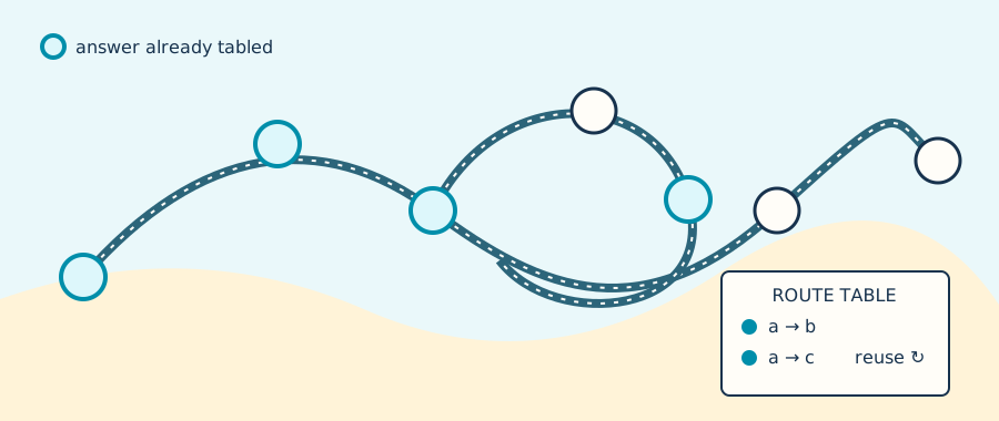
Tabling does not make every open relation finite. A rule that constructs ever-larger terms can still produce infinitely many distinct calls or answers. Keep the selected query and its generators finite.
A relation can construct a witness:
:- use_module(library(lists)).

path(X, Y, [X, Y]) :- edge(X, Y).
path(X, Z, [X | Rest]) :-
  edge(X, Y),
  path(Y, Z, Rest).
On cyclic graphs, track visited vertices and use ISO negation as
\+ member(Next, Visited) to obtain finite simple paths rather than arbitrary walks.
Notice that ancestor/2 and path/3 make different promises. Endpoint
reachability has at most one logical pair for each pair of vertices, whereas
path construction may have many witnesses for the same endpoints. Table the
finite relation you need; bound or simplify the richer witness relation. This
distinction reappears in grammars, planning, proof search, and program analysis.
Checkpoint. In the three-edge family from Chapter 1, predict the direct and
indirect ancestor/2 answers. Point to the base clause and recursive clause,
then say what becomes smaller or moves closer to a known fact in one successful
derivation.
5. Lists as relations
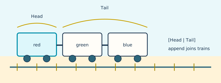
[a, b, c] abbreviates nested cons cells. [Head | Tail] exposes one cell;
[] is empty.
first([Head | _], Head).

contains_item(X, [X | _]).
contains_item(X, [_ | Rest]) :- contains_item(X, Rest).

joins([], Ys, Ys).
joins([X | Xs], Ys, [X | Zs]) :- joins(Xs, Ys, Zs).
Different modes give joins/3 different uses. It can construct a concatenated
list, enumerate every prefix/suffix split, or find a missing part. This is the
practical meaning of a relational definition.
Some algorithms carry explicit state through an accumulator:
reverse_acc(List, Reversed) :- reverse_go(List, [], Reversed).
reverse_go([], Acc, Acc).
reverse_go([X | Xs], Acc, Reversed) :-
  reverse_go(Xs, [X | Acc], Reversed).
No mutation occurs; every call receives a new term. EyeProlog also includes
member/2, append/3, select/3, nth0/3, reverse/2, length/2,
ISO sort/2, slicing helpers, and numeric summaries. Improper lists such as
[a | Tail] are valid terms, but operations requiring a proper finite list
fail unless the tail is [].
Checkpoint. Trace joins([a], [b, c], Whole) by hand. Then reverse the
question: bind Whole to [a, b, c] and predict all prefix/suffix splits.
Finally explain why [a | Tail] is not yet known to be a proper finite list.
Part I summary
Part I established the relational eye:
- a program is a theory of ground sentences, not a sequence of assignments;
- variables acquire meaning through consistent substitution;
- unification connects a question to facts and rule heads by structure;
- every rule has both a declarative and an operational reading;
- recursion describes an unbounded family of finite proofs;
- lists are inductive terms whose relations can support several modes.
You should now be able to read a program aloud, predict a unifier, write base and recursive clauses, and explain why a list relation may construct as well as inspect its arguments. Carry forward one habit: begin with a meaningful ground instance, then ask which variables may safely replace which parts.
Historical note: clauses become a programming medium
The ingredients of Part I were assembled across several traditions. First-order logic supplied variables, substitution, and quantified formulas. Herbrand made ground terms and ground instances central to proof theory. Robinson’s 1965 resolution principle gave automated deduction a uniform, machine-oriented inference rule whose practical force depended on unification.
Prolog emerged when these ideas met a natural-language project in Marseille in the early 1970s. Colmerauer and Roussel stress that the project did not begin as an abstract attempt to invent a programming language: the need to analyze French drove the development of executable clauses and their control. Lists then became more than containers. They naturally represented sentences, syntax, proof states, and sequences of goals. The familiar two-clause list program condenses a much older mathematical pattern—definition by constructors and structural induction—into executable form.
Part II — Search

A theory may justify many conclusions, but an evaluator must still find them. This Part studies the finite domains, constraints, failure, and choice that turn a field of possibilities into a productive computation.
6. Arithmetic and finite generation
Arithmetic uses the standard is/2 predicate, conventionally written with
infix operator syntax:
:- use_module(library(lists)).

next(X, Y) :- (Y is X + 1).
area_rectangle(W, H, Area) :- (Area is W * H).

hypotenuse(A, B, C) :-
  (A2 is A * A),
  (B2 is B * B),
  (C2 is A2 + B2),
  (C is sqrt(C2)).
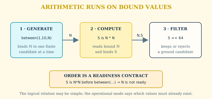
Inputs must be bound to suitable numbers before a numeric function runs. Comparisons filter generated solutions:
safe_reading(Sensor, Value) :-
  reading(Sensor, Value),
  (Value >= 0),
  (Value =< 80).
between(Low, High, Value) enumerates an inclusive integer range or checks an
already-bound value:
:- use_module(library(lists)).

square(N, Square) :-
  between(1, 10, N),
  (Square is N * N).
Finite generators turn loops into searches. Recurrences need intended modes:
factorial(0, 1).
factorial(N, F) :-
  (N > 0),
  (Previous is N - 1),
  factorial(Previous, PF),
  (F is N * PF).
The intended call direction belongs in the predicate’s tests and surrounding documentation; it does not require executable metadata.
Checkpoint. For every arithmetic goal above, mark which arguments must be
numbers before the goal can run. Explain why between/3 is a generator in
square/2 but merely a check when its third argument is already bound.
7. Failure, negation, and quantification
A goal fails when no clause or built-in proves it under current bindings. Failure prunes that branch and search tries another choice.
Failure is an operational event, not automatically a statement about the
world. Turning failure into \+ Goal is justified only relative to the
program and the current bindings. This is the closed-world move familiar
from databases: for some bounded relation, what cannot be derived is treated
as absent. It differs from the open-world stance common on the Web, where a
missing claim may simply be unknown. Neither stance is universally right; the
modeler must say which knowledge boundary is complete.
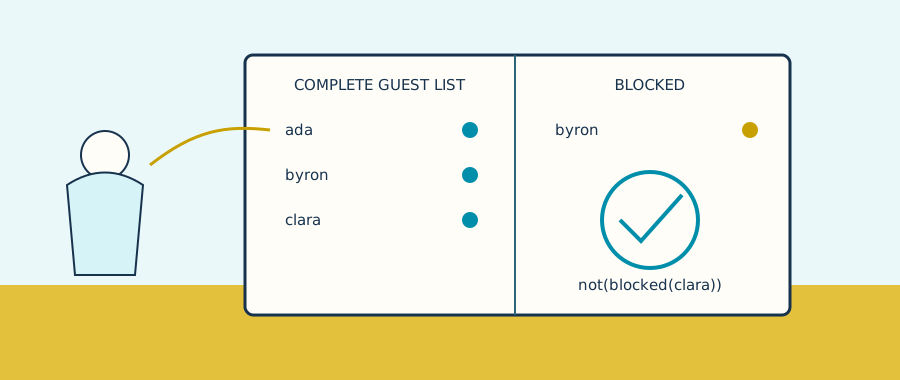
\+ Goal succeeds when Goal has no solution:
allowed(User) :-
  user(User),
  \+ blocked(User).
This means “blocked cannot be proved from this program,” not classical
negation. Bind variables before negating. Putting \+ blocked(User) before
user(User) asks whether there is no blocked user at all, not whether this
particular user is unblocked.
For ordinary \+/1, negative dependencies should normally be stratified:
compute a lower relation, then negate it from a higher layer. Use --warnings
to report negative recursion:
eyeprolog --warnings program.pl
Some finite rule systems intentionally contain recursion through negation. In
normal mode, EyeProlog provides explicit tnot/1 for that case. When the
reachable component is finite, function-free, and range-restricted Datalog,
cycles through tnot/1 are evaluated with the well-founded semantics (WFS)
rather than ordinary negation-as-failure. WFS has three truth states: true,
false, and undefined. A negative cycle may therefore leave the query
undefined instead of forcing an arbitrary true/false choice.
move(a, b).
move(b, a).
win(X) :- move(X, Y), tnot(win(Y)).
Here neither win(a) nor win(b) is unconditionally established; both belong
to the undefined part of the well-founded model. EyeProlog retains that
undefined state internally, but it does not treat an undefined atom as a
successful query answer, nor does it continue evaluating the rest of a
conjunction as though that atom had succeeded.
Use wfs_truth/2 when the truth state itself is data:
?- wfs_truth(win(a), Truth).
   Truth = undefined.
The inspected goal must be ground. The predicate reports true, false, or
undefined; reporting undefined is a successful result of wfs_truth/2, not
a successful execution of the inspected goal.
Direct calls to tnot/1 must be ground. In WFS rules, variables occurring in
the head or a negated literal must be range-restricted by positive body
literals. Ordinary \+/1 is unchanged, and strict ISO mode does not provide
tnot/1.
Universal checking needs no extension predicate: define the counterexample and negate it.
all_tests_pass(Suite) :-
  \+ failing_test(Suite).

failing_test(Suite) :-
  test_in(Suite, Test),
  \+ passed(Test).
Use negation where the knowledge boundary is closed: a complete roster,
configuration, or finite result set. In open-world data, model explicit states
such as confirmed_absent instead of deriving absence from silence.
Checkpoint. Compare user(User), \+ blocked(User) with
\+ blocked(User), user(User). State the question each ordering asks and the
completeness assumption needed before calling either result “allowed.”
8. Collecting and choosing answers
Finite aggregation asks about a solution set:
:- use_module(library(aggregate)).
:- use_module(library(lists)).
:- use_module(library(iso_ext)).

findall(Template, Goal, List).
countall(Goal, Count).
sumall(Value, Goal, Sum).
:- use_module(library(aggregate)).
:- use_module(library(lists)).

outgoing_costs(Node, Costs) :-
  findall(Cost, edge(Node, _, Cost), Costs).

total_outgoing(Node, Total) :-
  sumall(Cost, edge(Node, _, Cost), Total).
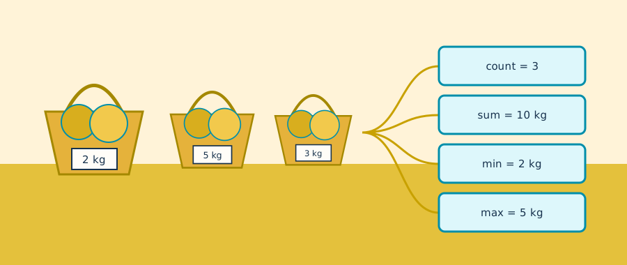
findall/3 returns [] for no answers; counts and sums return zero.
Choose a collector from the question, not from convenience:
| Question | Result shape | Empty search |
|---|---|---|
| Which witnesses were found? | findall/3 returns a list |
[] |
| How many derivations succeeded? | countall/2 returns an integer |
0 |
| What is their numeric total? | sumall/3 returns a number |
0 |
| Which candidate has the least or greatest key? | aggregate_min/5 or aggregate_max/5 returns one candidate |
failure |
Counting solutions is not necessarily counting distinct domain objects: two
proofs may resolve the visible value in the same way. When identity matters,
collect the identifying template and deliberately canonicalize it with ISO
sort/2; when derivation multiplicity matters, retain the duplicates. Making
that decision explicit prevents a database-style summary from silently
changing the question.
Optimization can retain only a best solution:
:- use_module(library(aggregate)).
:- use_module(library(lists)).

best_route(From, To, Route, Cost) :-
  aggregate_min(
    [CandidateCost, CandidateRoute],
    CandidateRoute,
    route(From, To, CandidateRoute, CandidateCost),
    [Cost, Route],
    Route
  ).
The key [Cost, Route] supplies deterministic tie-breaking through term order.
aggregate_min/5 and aggregate_max/5 fail when their goal has no answers.
An aggregate opens a smaller query scope inside the surrounding proof, and its
inner search must be finite.
Keep candidate generation separate from choice. A relation such as
route/4 should explain which routes exist and how their costs arise;
best_route/4 states a policy over that finite relation. This separation lets
the same candidates be inspected, counted, tested, or optimized without
burying their meaning in a single committed search. It also makes an empty
candidate set visible: “there is no route” is different from inventing a
sentinel route with an artificial cost.
Checkpoint. For an empty route relation, predict the behavior of
findall/3, countall/2, sumall/3, and aggregate_min/5. Then identify the
finite generator that bounds each aggregate in a program of your own.
9. Structured data, text, and contexts
Term predicates decompose or construct general terms:
functor(Term, Name, Arity).
arg(Index, Term, Value).
(Term =.. [Name | Arguments]).
arg/3 uses one-based indexes. Prefer direct pattern matching when the shape
is known; use inspection for generic transformations.
Text is best normalized at the model boundary. The library(strings) module
uses ISO-friendly atoms or proper lists of one-character atoms for its text
arguments; newly produced text is an atom:
:- use_module(library(strings)).
:- use_module(library(lists)).

normalized(Input, Words) :-
  trim(Input, Trimmed),
  lowercase(Trimmed, Lower),
  split(Lower, ' ', Words).
Conversions include number_string/2, atom_string/2, and term_string/2.
Pattern operations include contains/2, matches/2, and named-capture
matches/3. Turn text into structured terms early and keep central rules
relational. Double-quoted source notation follows the ISO double_quotes flag;
it does not create a separate Prolog string type.
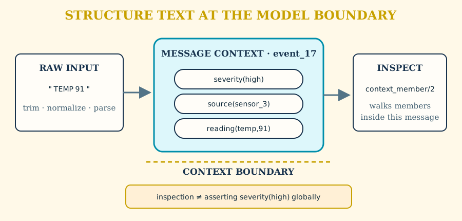
Parenthesized comma terms can serve as context data:
:- use_module(library(lists)).

message(event_17, (severity(high), source(sensor_3), reading(temp, 91))).

context_member((Left, _right), Member) :- context_member(Left, Member).
context_member((_left, Right), Member) :- context_member(Right, Member).
context_member(Member, Member) :- Member \= (_left, _right).

hot_event(Id) :-
  message(Id, Context),
  context_member(Context, severity(high)),
  context_member(Context, reading(temp, Value)),
  (Value > 80).
context_member/2 is an ordinary program relation: it walks a comma-context
from left to right. When the member’s shape is not known in advance, decompose
it with (Member =.. [Name | Arguments]). Context members remain quoted data;
inspecting them does not assert them as ambient facts.
Checkpoint. Distinguish the atomic formula message(...) from the nested
data term (severity(high), source(sensor_3), reading(temp, 91)). Explain why
context_member/2 can inspect the latter without asserting severity(high)
globally.
10. From puzzles to models
A robust finite search has three layers: generate candidates, constrain them, and present a concise answer.
color(red).
color(green).
color(blue).

coloring(A, B, C) :-
  color(A),
  color(B),
  (A \= B),
  color(C),
  (B \= C),
  (A \= C).

answer(colors(A, B, C)) :- coloring(A, B, C).
eyeprolog --goal 'answer(X)' program.pl
Place cheap, selective constraints as soon as their inputs are bound. For state-transition problems, represent state and moves explicitly:
:- use_module(library(lists)).

plan(State, State, _, []).
plan(State, Goal, Seen, [Move | Moves]) :-
  transition(State, Move, Next),
  \+ member(Next, Seen),
  plan(Next, Goal, [Next | Seen], Moves).
The visited list makes a finite state space explicit. EyeProlog is strongest when the result is a logical consequence with a compact witness: a path, matching, classification, schedule, proof, or bounded model. Mutable arrays and large numerical kernels generally belong in a host, with EyeProlog as the decision layer.
For the coloring program, the six printed answers are the permutations of
red, green, and blue:
answer(colors(red, green, blue)).
answer(colors(red, blue, green)).
answer(colors(green, red, blue)).
answer(colors(green, blue, red)).
answer(colors(blue, red, green)).
answer(colors(blue, green, red)).
Checkpoint. Label the generator, each constraint, and the final witness in
the coloring program. Before changing it, predict how many answers remain if
A \= C is removed; then run the program and account for every additional
answer.
Part II summary
Part II turned relations into finite computations:
- arithmetic relations need their operational inputs bound;
- generators state where finite candidates come from;
- failure prunes a branch, while
\+/1makes finite failure a closed-world test; - recursion through negation is handled by
tnot/1and the well-founded semantics, whose undefined truth state is retained rather than forced; - aggregates turn a finite solution space into a list, count, sum, or optimum;
- structured terms and contexts belong at explicit modeling boundaries;
- puzzles become programs by separating generation, constraint, and witness.
You should now be able to justify a query’s finiteness, order goals by binding dependency, distinguish negation as failure from classical negation, and explain why optimization is search plus an ordering.
Historical note: control, databases, and finite failure
Early Prolog made a decisive engineering choice: clauses would be tried in an order and subgoals would normally be selected left to right. That choice made logic executable, but also made control visible. A logically symmetric conjunction could behave asymmetrically when one order supplied a value and another asked arithmetic to run too soon.
The meeting of logic programming and database research in the 1970s sharpened questions about finite relations, closed-world reasoning, and query evaluation. Keith Clark’s 1978 account did not identify failure with unrestricted logical negation; it related negation as failure to a completed database reading. Later work on stratification disciplined negative dependencies. Aggregation continued the database lineage: a set of solutions could itself become data, provided the nested search was finite.
These distinctions explain EyeProlog’s conservative treatment. Negation and aggregation are powerful because they expose a bounded subcomputation. Their safety comes not from punctuation but from a mathematical argument about scope and termination.
Part III — Trustworthy reasoning
An answer becomes useful when its grounds remain visible. Here reasoning is treated as an accountable structure: queries define the question, proofs retain support, integrity checks expose invalid states, and knowledge boundaries stay explicit.
11. Queries, answers, and proofs
EyeProlog goals are supplied by the host, for example
eyeprolog --goal 'child(X, Y)' program.pl. EyeProlog prints ground answers, removes
duplicates, and suppresses answers that merely repeat source facts. Answers
are not inserted back into the running program.
An answer and a derivation serve different audiences. An answer records what the theory supports; a derivation records how this run supported it. In mathematics that distinction resembles theorem versus proof. In data systems it resembles result versus provenance. The proof is not a substitute for valid source data or sound domain rules, but it makes both reviewable: a user can trace a decision to clauses, facts, bindings, and built-in operations instead of trusting an opaque status code.
Use --proof or -p to add the derivations to the result document:
eyeprolog --proof examples/socrates.pl
type(socrates, mortal).

clause(1, type(socrates, man), true).
clause(2, type(var('X'), mortal), type(var('X'), man)).

step(type(socrates, mortal), rule(2), ['X' = socrates], [type(socrates, man)]).
step(type(socrates, man), fact(1), [], []).
A proof states what was concluded and then why: the claims first, then the
clause/3 records the derivations cite and one step/4 fact per justified
conclusion. That is the same division eyeron, eyeling and eyeleng make –
there the claims are derived triples and the steps carry pe:rule. Proof
output is valid EyeProlog input and can be kept and checked later:
eyeprolog --proof examples/socrates.pl > socrates.why.pl
eyeprolog --check-proof socrates.why.pl examples/socrates.pl
The second command re-performs every inference the document records against the program; it does not search again for a proof. A changed source clause, a changed use, or a changed recorded binding makes the check fail. Proof input is parsed as Prolog data rather than loaded as a program, so its terms cannot trigger directives while being checked.
Enabling --proof, --warnings, or --stats must not change which answers
are found.
A step has the shape step(Conclusion, By, Bindings, Uses): what was
concluded, the single term saying why it holds, the bindings that
justification used as 'Name' = Value pairs, and the conclusions it used.
Those four parts in that order are what eyeron, eyeling and eyeleng write too
— pe:rule, pe:binding and pe:uses in the two RDF syntaxes — so one
reading serves the whole family, and a use is named by its own conclusion
rather than by an id to be joined back, which lets a proof be read downward
from the claim.
A resolution proof is a tree in which the same goal may be proved more than
once — the two q(1) subproofs of p(ok) :- q(1), q(1). are the plain case —
but the document is flat: each conclusion gets one step, however many
derivations reach it, and that step is the first one found. A proof therefore
grows with the number of distinct conclusions, not with the shape of the
search.
By is rule(N) or fact(N) citing a clause/3 record, or builtin,
absent or collected for a built-in goal, a completed \+ or a completed
findall/3. A clause is numbered by its position in its own source file, not
by its position in the running database, so assert/1 and retract/1 cannot
move what a citation means; a clause asserted at run time is in no source file
at all and is recorded as asserted. A bundled library’s clauses are not the
program’s own, so a step through one is recorded as builtin;
--proof-detail expanded still explains through a library predicate rather
than stopping at it. Explanation data is outside the logical semantics of the
input program: it describes the derivation but does not participate in finding
it.
Checking re-performs each step against the clause it cites: the clause must
exist, its variables bound as the step recorded them must yield exactly this
conclusion from exactly these uses, every claim must have a step, every use
must resolve to a step or to a statement the program gives, and no conclusion
may rest on itself. A builtin step derives from no clause, so reading the
document cannot decide it; it is computed again instead, against a program
holding the bundled libraries and no clause of the theory under proof, and
must agree. absent, collected and asserted steps stay trusted: the first
two range over the theory that recomputation deliberately excludes, and a
clause asserted at run time is in no source file to check against. The report
counts what was verified, what was recomputed, and what remains an obligation
rather than folding them into an undifferentiated success. An
answer the solver found but the explanation cannot reproduce is recorded as
unproven, which makes the document fail its check, because that is the
truth about it.
A second program can query these facts. Read a proof as an argument. If it contains irrelevant detours, improve the helpers. If a key premise is hidden inside an opaque value, model it as a fact. Designing for a good explanation often produces a better theory.
Checkpoint. Run examples/socrates.pl once normally and once with
--proof. Confirm that the ground answers are unchanged. In one proof,
identify the queried goal, the rule that derived it, the source fact used, and
the binding carried between them.
12. Integrity checks as ordinary predicates
Integrity conditions are ordinary relations that describe invalid input states:
invalid_probability(Disease, Probability) :-
  probability(Disease, Probability),
  (Probability > 1).
A host that requires validated input queries the integrity relation explicitly before it asks for domain decisions. This keeps the policy visible: the host may reject the input, report every defect, or continue in a diagnostic mode.
false/0 keeps its ISO meaning: it is a built-in goal that always fails. It is
a protected static procedure, so false. and clauses of the form
false :- Body. are rejected with
permission_error(modify, static_procedure) rather than acquiring special
pre-query behavior.
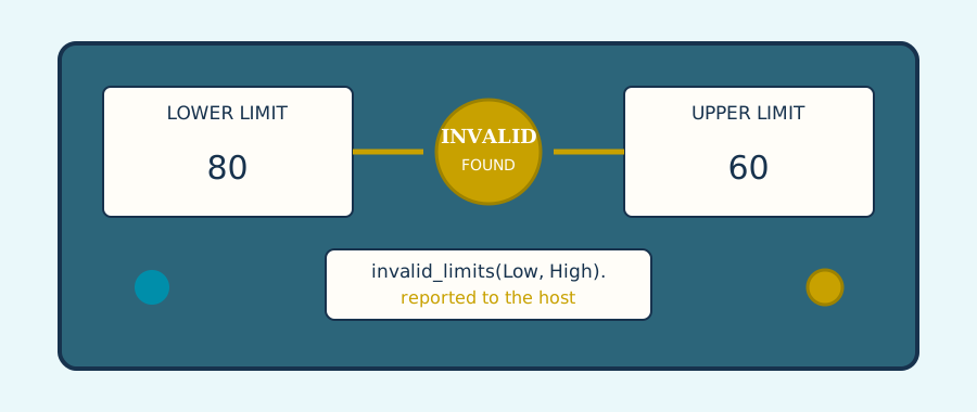
invalid_assignment(Person, Role, Other) :-
  assigned(Person, Role),
  incompatible_roles(Role, Other),
  assigned(Person, Other).
The logical reading is that the program can derive witnesses for an inadmissible combination. The operational response is outside the relation itself and remains an explicit host decision.
Designing an integrity relation
Start with a sentence that must never be accepted, then translate its witnesses into positive, finite goals. “No person has two incompatible roles” becomes the relation above. A useful integrity check is:
- domain-specific: it names an impossible or inadmissible state;
- finite: its intended validation query can be checked completely;
- diagnostic: its arguments identify the offending records; and
- explicit: callers can choose whether to reject, report, or inspect defects.
Four outcomes that can look like “failure” at a shell prompt have different meanings:
| Outcome | Interpretation | Appropriate response |
|---|---|---|
| query has no answer | this theory did not derive the selected goal | inspect data, rules, and closed-world assumptions |
| integrity query has an answer | the supplied input contains a forbidden combination | repair, reject, or report the input |
| resource ceiling is reached | the computation exceeded an operational budget | bound or redesign the search |
| parser or type error | the program or call violates the language contract | correct the source or interface |
Do not treat every undesirable business result as invalid input. A declined application, unavailable route, or negative test may be a perfectly valid answer of the theory. Reserve integrity relations for states whose witnesses must be handled before trusted downstream decisions.
To see the explicit validation path, run:
eyeprolog examples/integrity-check.pl
It prints the invalid-state witness and the resulting diagnostic status. Nothing runs implicitly before the supplied goals.
Checkpoint. Explain the difference between an ordinary query with no answer and an integrity query that returns a defect. Write one invalid-state relation and one ordinary negative result that should remain query failure.
13. Termination, tabling, and performance
Declarative clarity and operational care reinforce each other. Bind selective arguments early, keep generators finite, and make decreasing structure visible.
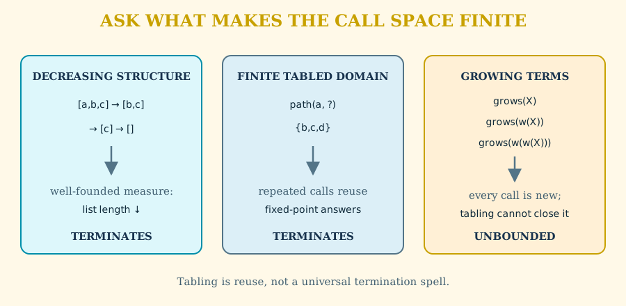
Naive depth-first search can revisit the same recursive question indefinitely. Tabling changes the unit of work: a call pattern becomes a shared subproblem, its answers are remembered, and consumers reuse answers rather than expanding the same call again. This idea connects logic programming to memoization and dynamic programming, but tabling also has a semantic role: over a finite positive recursive domain, repeated rounds can compute the least fixed point. It is therefore especially natural for reachability, grammars, dependency analysis, and other recursive relations with overlapping subproblems.
Ordinary goals, including recursive ones, use indexed depth-first resolution. Tabling is opt-in: declare a predicate with :- table p/n. when its
recursive calls should share answers and cyclic calls should iterate toward a
fixed point. For sufficiently large finite, function-free Datalog dependency
cones rooted at an explicitly tabled predicate, EyeProlog may share one
most-general relation table across call variants. This turns an open closure
such as tc(X, Y) into one finite relation computation rather than many
overlapping bound subcomputations; bound consumers can then use indexes over the
stored answers. The declaration is the language-level choice; how a declared
table is represented and indexed remains an engine optimization.
Recursive components with negative dependencies are not positive least-fixed-
point problems. When such a component uses explicit tnot/1 and satisfies the
finite, range-restricted, function-free Datalog restrictions, EyeProlog instead
computes the alternating fixed point of the well-founded semantics. Existing
\+/1 code remains ordinary negation-as-failure.
Deeper implementation: how clause indexing stays semantic
This section explains why an optimization does not change clause meaning. Readers focused on modeling may skip to the statistics command and return when performance or implementation portability becomes relevant.
Every predicate group keeps compact indexes for scalar values in each argument
position. Index keys include the scalar type, so 7, '7', and "7" remain
distinct even though their printed payload is the same. A clause whose indexed
head argument is a variable or structured term
stays in a fallback set, and the selected candidates are merged back into
source order before unification. An index narrows where to look; it never
decides whether a clause matches.
For groups of at least ten clauses, a call with several bound scalar arguments may cause a wider combined index to be built on demand. The admission policy rejects indexes with too many variable fallbacks or too little expected speedup, and requires a combined index to improve substantially over the best single-argument index. These choices are performance details: removing every index should change running time, not answers or clause order.
Authors choose query modes, finite domains, visited-state representations, negation strata, and witness size. They normally do not choose the engine’s search strategy.
Inspect counters without changing answer output:
eyeprolog --stats examples/observability-log-correlation.pl
The reported counters include completed goal lists, calls to the goal solver
and single-goal solver, unification attempts, maximum depth and goal-list size,
deterministic built-in successes and failures, and table fixed-point rounds.
WFS execution additionally reports wfs_fixpoint_rounds and
wfs_undefined_answers. The latter counts undefined atoms encountered while
resolving query goals; it is an execution statistic, not a declaration
that those atoms are true. All statistics describe work performed, not logical
truth. Compare counters only across equivalent queries and the same
implementation version.
Common sources of nontermination are recursive calls made before constraints, ever-growing terms, infinite open mathematical queries, negative cycles, and path enumeration without a visited set. Repair the model by strengthening the query, adding a finite domain, tracking states, or exposing a decreasing argument.
Checkpoint. Classify three recursive calls: one justified by a decreasing list, one by finitely many tabled graph answers, and one that constructs terms without bound. State why the first two may terminate and why tabling does not repair the third.
Eyelet forward rules and Prolog execution
EyeProlog normal mode also accepts :+ at priority 1200 as an xfx operator.
A source term
Conclusion :+ Premise.
is a forward rule. When a loaded program contains such rules and no explicit
top-level goal overrides them, the engine loads library(eyelet) and invokes its
Prolog closure driver. The driver inspects :+/2 clauses structurally, prepares
state predicates for updates, repeatedly solves premises against the current
program, asserts novel conjuncts from successful conclusions, and continues until
no new conclusion is added. Query-only programs take a single-pass fast path
because they cannot grow the closure. This is the execution path used when Eyelet
sources are run directly by EyeProlog.
Two conclusions have control meaning. true :+ Goal is a query and prints each
distinct successful instance of Goal. false :+ Goal is an integrity fuse:
on success EyeProlog prints fuse(Goal) and returns halt status 2. Variables
that occur only in an ordinary derived conclusion are existential and become
sk_0, sk_1, and so on; a derived conclusion that is itself a :+ rule keeps
its variables universal. The driver uses an explicit changed marker to repeat
only productive rounds. stable(Level) raises the requested closure level and
succeeds once that level has been reached. becomes(From, To) performs linear
state replacement and prepares existing user predicates for mutation, so an
EyeProlog source does not need a separate dynamic/1 declaration merely to use
that state with becomes/2.
The :+ reasoning algorithm is therefore Prolog code in src/lib/eyelet.pl, not
a second JavaScript implementation. The remaining JavaScript references have
non-semantic roles: the parser declares the normal-profile operator, program
analysis scans forward-rule premises for dependency/autoload planning, execution
bootstraps the private eyelet:eyelet_run/3 entry point, and two private library
adapters bridge database mutability and answer/fuse events to the host. Those
adapters are not part of the strict ISO registry or the public library(eyelet)
export surface.
The JavaScript convenience run() function selects this forward mode when no
explicit goal or goals option is supplied. Advanced embedders can inspect a
parsed program with hasForwardRules(program) and invoke
executeForwardRules(program, solver, callbacks) directly. Strict ISO mode
removes the :+ operator and does not execute this extension.
Resource bounds are never logical answers. Normal execution has no implicit
depth limit. If an embedder explicitly supplies maxDepth and the search
exceeds it, EyeProlog raises resource_error(depth_limit) instead of silently
turning that branch into failure. Tabling is never selected implicitly: ordinary
recursive predicates retain standard depth-first Prolog control, and only a
source-level :- table p/n. declaration opts a predicate into fixed-point tabled
execution.
14. Knowledge engineering
A maintainable theory separates:
- source facts: measurements, records, and asserted relationships;
- helpers: normalization, classifications, and reachability;
- decisions:
status/2,action/2,risk/2, andreason/2; - integrity relations: predicates that return diagnostic invalid-state witnesses;
- outputs: focused host-supplied goals.
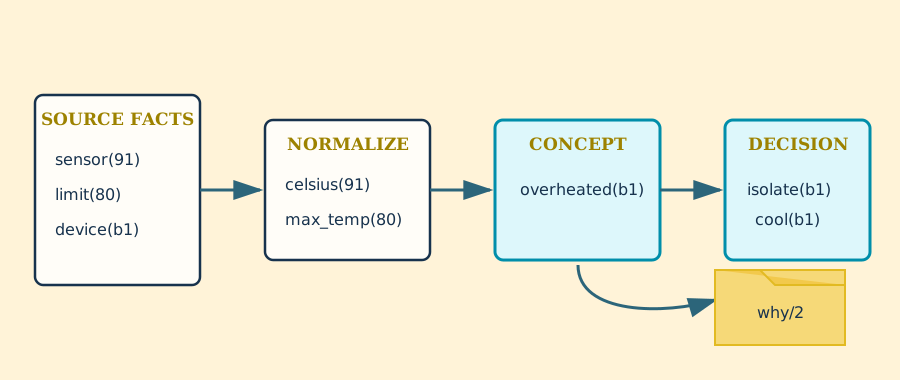
Prefer positive domain concepts. Use negation only across a closed boundary. Represent confidence, alternative worlds, and provenance explicitly rather than hiding them in rule order.
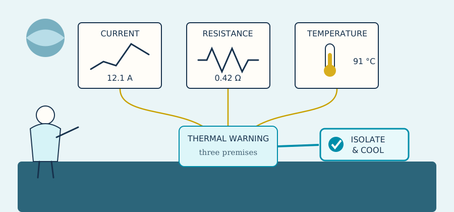
An evidence-backed diagnosis can separate physics from policy:
heating(Battery, Watts) :-
  current(Battery, Amps),
  resistance(Battery, Ohms),
  (I2 is Amps * Amps),
  (Watts is I2 * Ohms).

thermal_warning(Battery) :-
  heating(Battery, Watts),
  heating_limit(Limit),
  (Watts > Limit),
  temperature(Battery, Celsius),
  temperature_limit(TLimit),
  (Celsius > TLimit).

action(Battery, isolate_and_cool) :- thermal_warning(Battery).
Physics, limits, redundant sensing, and policy become distinct proof steps. See
examples/spacecraft-battery-diagnosis.pl for a complete case.
Test theories with successful derivations, expected failures, boundary values, duplicate paths, contradictory inputs, and proof premises. The repository’s conformance cases, example goldens, and proof goldens demonstrate these levels.
Checkpoint. Draw four columns for the battery example: source, physical concept, decision, and integrity. Place each predicate in a column, then list the measurements and policy thresholds that a proof cannot authenticate by itself.
15. Explicit data boundaries
EyeProlog deliberately keeps external integration outside the reasoning core. An embedder validates input, converts it to ordinary Prolog terms and clauses, and then asks the solver a focused goal. This keeps parsing a business format, authenticating a source, and deriving a conclusion as three separate jobs.
A boundary should make four decisions visible:
- which external values are accepted;
- how they map to finite Prolog terms;
- which predicates the imported clauses may define; and
- which resource limits apply to the resulting query.
A boundary in four steps
Suppose a host receives one JSON temperature record. The host, not the logic program, owns the JSON syntax and the decision to trust that record. A narrow adapter can validate the record, map its values into a deliberately small Prolog vocabulary, construct the theory, and ask one bounded question:
import { run } from 'eyeprolog';

const inputText = '{"sensor":"sensor_1","celsius":91}';
const allowedSensors = new Set(['sensor_1', 'sensor_2']);

function reasoningSource(record) {
  if (!record || typeof record !== 'object') throw new TypeError('record');
  if (!allowedSensors.has(record.sensor)) throw new TypeError('sensor');
  if (!Number.isFinite(record.celsius)) throw new TypeError('celsius');
  if (record.celsius < -100 || record.celsius > 200) {
    throw new RangeError('celsius');
  }

  return `
reading(${record.sensor}, ${record.celsius}).
thermal_alert(Sensor) :-
  reading(Sensor, Celsius),
  (Celsius >= 80).
`;
}

const record = JSON.parse(inputText);
const result = run(reasoningSource(record), {
  goal: `thermal_alert(${record.sensor})`,
  proof: true,
  maxDepth: 10_000,
  maxInferences: 100_000,
  maxMemoryBytes: 256 * 1024 * 1024,
  solutionLimit: 10
});

console.log(result.stdout);
The allow-list makes interpolation safe here: the external sensor identifier
can become only one of two known Prolog atoms, and the temperature must be a
finite number in an accepted range. General text must be encoded with a
well-tested term constructor or serializer rather than inserted into source.
The generated program defines only reading/2 and the fixed domain rule; the
host supplies the goal and ceilings explicitly.
This small example exposes four different claims:
| Stage | Claim and owner |
|---|---|
| Parse | the bytes are valid JSON — host parser |
| Validate | the record has an accepted sensor and temperature — adapter |
| Convert | the accepted values denote these exact Prolog terms — adapter |
| Derive | the supplied reading satisfies thermal_alert/1 — EyeProlog proof |
The proof procedure can explain how supplied clauses support an answer. It cannot prove that a file, database, sensor, or remote service was trustworthy. That responsibility stays with the host application.
Checkpoint. Choose one external record used by an application. State what the host validates, the Prolog term it constructs, the goal it asks, and the resource limit that prevents an untrusted input from consuming unbounded work.
16. Embedding EyeProlog
The JavaScript API exposes a convenience runner and lower-level types:
import { run, Program, Solver, parseGoalText } from 'eyeprolog';

const result = run(`
answer(ok) :- ok = ok.
`, { goal: 'answer(X)' });
console.log(result.stdout);
console.log(result.stats);
The first console.log prints answer(ok). followed by a newline. The second
prints numeric work counters; those counters describe this run rather than an
additional logical answer.
run/2 accepts source text or an already parsed Program. Its options include
proof (with why and explain as aliases), proofDetail (abstract or
expanded), maxDepth, maxInferences, maxMemoryBytes, solutionLimit, a
custom registry, and strictNegation or analyzeNegation. It returns
stdout, the solver’s numeric stats, and a nullable haltCode; it does not
write to the process streams.
For applications that exchange proofs independently of answer output, the same
module exposes proofCertificate(program, goal, options),
proofCertificatesFromText(text, program), and
verifyProof(program, certificate, options):
import {
  Program, parseGoalText,
  proofCertificate, proofCertificatesFromText, verifyProof
} from 'eyeprolog';

const program = Program.parse(`
p(a).
q(X) :- p(X).
`, { sourceMetadata: true });

const made = proofCertificate(program, parseGoalText('q(a)'));
console.log(verifyProof(program, made).ok); // true

const received = proofCertificatesFromText(made.text, program)[0];
console.log(verifyProof(program, received).ok); // true
proofCertificate returns both the ordinary why/2 text and a JSON-serializable
certificate object. verifyProof walks the supplied certificate rather than
asking the solver to find another proof; its trusted array lists every builtin
or abstract-library boundary that was assumed while checking it. Passing
proofDetail: 'expanded' exposes bundled Prolog-library clauses in the
certificate and therefore reduces library-level trust boundaries to the
built-ins those clauses ultimately use.
When run receives an already parsed Program, bundled-library imports
needed only by its host-supplied goals are added to that Program before solving,
just as they are while source text is parsed. The autoload index covers every
exported predicate in the bundled src/lib/ modules. Pass autoload: false
when the Program must retain only explicitly imported predicates.
For applications that inspect or prepare a theory before running it, use
Program directly:
const source = `
edge(a, b).
edge(b, c).
path(X, Y) :- edge(X, Y).
path(X, Z) :- edge(X, Y), path(Y, Z).
`;

const program = Program.parse(source, { analyzeNegation: true });
const goal = parseGoalText('path(a, X)');
const path = program.findGroup('path', 2);

console.log(goal);
console.log(program.stratifiedNegation);
console.log(path?.recursive, path?.tabled, path?.tableInputPositions);

const solver = new Solver(program, {
  maxDepth: 50_000,
  maxInferences: 1_000_000,
  maxMemoryBytes: 256 * 1024 * 1024,
  solutionLimit: 100_000
});
The limits are safety ceilings, not logical declarations. Reaching the depth,
inference, or solution ceiling may truncate search; it does not prove that no
further answer exists. Reaching maxMemoryBytes instead raises
resource_error(memory), because continuing until the JavaScript engine’s hard
heap limit would let the host abort before Prolog could report an exception. At
the Solver API boundary, solutionLimit is opt-in: if it is omitted, ordinary
solving and child searches that inherit the solver limit do not stop after a
fixed number of solutions. This matters for re-executable goals such as
repeat/0 and for library relations such as call_nth/2; an implementation
safety threshold must not turn a still re-executable search into logical
failure. Embedders that need a finite answer budget should pass solutionLimit
explicitly.
Variable term order is deliberately scoped rather than stored as a permanent
property of a variable. ISO 13211-1 section 7.2.1 leaves the order of two
distinct variables implementation dependent and requires constancy only while
a sorted list is being created. EyeProlog therefore chooses a local variable
ranking for an ordinary term comparison, while sort/2, keysort/2, and the
sorting step of setof/3 share one ranking for the duration of that single
sorted-list operation. No process-global variable registry or creation ordinal
is retained or exposed through later comparisons.
EyeProlog periodically checks detectable JavaScript heap use and keeps a quarter
of the applicable host heap ceiling in reserve so the solver can unwind and report
resource_error(memory) before a fatal host out-of-memory abort. When Node is
started with --max-old-space-size, the guard compares that old-generation
ceiling with V8’s non-young heap spaces; short-lived new-generation allocations
therefore do not cause a false resource error. Embedders may
replace that automatically derived soft ceiling with maxMemoryBytes; setting
it to Infinity disables the proactive check. Environments that do not expose
heap use cannot provide the proactive check. Host capacity failures that V8
reports as Map maximum size exceeded or Set maximum size exceeded are also
normalized at the solver boundary instead of leaking a JavaScript RangeError.
ISO 13211-1 leaves the resource atom implementation dependent. EyeProlog uses
memory for a finite host allocation/capacity ceiling and reserves the
finite_memory spelling for the distinct convention where no finite amount of
memory could complete the computation. After a recoverable memory error, the
solver keeps a bounded recovery window while the failed search unwinds so the
host can collect released query terms. The same solver can then run later
queries; this recovery does not resume the query that exhausted its limit.
The iterative solver keeps active-call frames only where they are semantically
needed for cut scope or recursive variant guards. Bundled-library helpers whose
callable dependency region is cut-free and which need no recursive variant
guard therefore do not copy a growing active-call sequence at every step.
Under the normal EyeProlog registry, the bundled Prologue length/2 also has a
scoped iterative execution path: named lists are counted or constructed without
recursive interpreter frames, and an anonymous list is not materialized because
its binding cannot be observed. A newly constructed fixed-length suffix starts
as a lazy compact skeleton and expands one ordinary ./2 cell at a time when
unification, another list predicate, or answer readback inspects it. This is a
storage optimization, not a distinct Prolog term or list semantics. Embedders
that inspect the JavaScript term model can recognize this representation with
CompactListTerm, isCompactList, and compactListLength, or construct one
with compactVariableList. For open-ended length(List, N) generation, each generated spine is known not
to contain the caller’s dereferenced tail variable. The bundled path passes that
proof through the normal unifier, sharing the same proven-nonoccurrence mechanism
as first-use clause variables instead of maintaining a predicate-specific raw
binding shortcut. It still reserves recovery headroom proportional to the
retained spine, so a finite heap limit is raised inside the length/2 search as
a catchable resource_error(memory) rather than allowing an outer solver frame
to encounter the limit first.
The same proven-nonoccurrence mechanism has a conservative source-level form for freshly renamed
clauses. A singleton variable in the clause head, or a variable that has not
appeared in the head or any earlier body goal and occurs exactly once in a
direct =/2 goal, cannot already be a subterm of the value it is about to
receive. EyeProlog marks only that binding as locally fresh and skips its occurs
traversal. A repeated variable such as the X in X = f(X), a variable already
seen earlier in the clause, and unify_with_occurs_check/2 all keep the normal
finite-tree check. The solver also treats such a first-use equality as a
source-order barrier for its deterministic-goal scheduling, so the freshness
proof cannot be invalidated by moving a later goal ahead of it. This recovers
much of the classic WAM-family “local variable” optimization for DCG tail
variables without introducing a WAM local/global stack distinction into the
JavaScript term model.
For grammar execution, phrase/2 passes its fixed final remainder [] directly
into the expanded grammar. Besides matching the two-argument contract, this
avoids repeatedly trying an empty production against a temporary output
variable. phrase/3 still uses a private final-output variable and delays its
last unification, preserving the existing steadfast treatment of its explicit
third argument. The ordinary length/2 clauses remain the authoritative module
definition and are used unchanged by the ISO-only registry and whenever delays
or finite-domain constraints require their normal wake-up points.
Implementation boundary
The source layout mirrors the language boundary while keeping the JavaScript
runtime flat under src/. src/iso.js remains the stable ISO facade and
built-in registry; arithmetic evaluation lives in src/iso-arithmetic.js, and
processor control/error classes live in src/errors.js. src/dcg.js
implements the shared Part 3-oriented grammar-rule and dynamic-body expansion
without depending back on the ISO registry. This keeps the low-level syntax and
error layers acyclic while preserving the existing src/iso.js exports.
src/cleanup.js is an execution-layer sibling of the solver. It installs
lifecycle-aware closing of protected builtin iterators from the supported API
and CLI entry paths and registers call_cleanup/2 and
setup_call_cleanup/3 for the normal EyeProlog profile. The standard-library
layer does not import the solver back through this module, preserving the
acyclic source graph.
Program preparation follows the same pattern. src/program.js remains the
Program facade and source/module loader. Static recursion, Datalog, WFS, and
negation-stratification analysis is isolated in src/program-analysis.js,
while compact-clause representation and conservative candidate indexes live in
src/program-indexing.js. The solver consumes those same indexes directly;
large execution fast paths deliberately remain in src/solver.js rather than
being split through extra strategy objects or callbacks. Architectural cleanup
is required to preserve performance as well as semantics.
Focused files under src/lib/ contain the portable extensions, with
src/lib/lists.pl supplying common list relations. They are ordinary Prolog modules using EyeProlog’s documented module compatibility
surface, organized like Trealla’s library/ and registered for
library(Name) by src/standard-library.js in Node and the browser. The
browser entry point src/playground-worker.js uses that same program and
module-loading path in a dedicated worker. src/ARCHITECTURE.md records the
layering and dependency rules, and the architecture regression rejects
JavaScript import cycles.
Normal CLI, JavaScript, Solver, proof replay, and the browser playground use
the same module loader. A library is added to a Program only when its source
uses use_module/1 or use_module/2; exported predicates are imported into the
calling module and private predicates remain module-local. Advanced embedders
and conformance tests can select getStrictIsoRegistry() together with
isoStrict: true for the Part 1 + Corrigenda strict surface. All paths share
the parser, term representation, solver, streams, and proof machinery.
Extending the built-in registry
An embedder can start from the default EyeProlog registry and add a host relation. A handler is a generator over environments. It should clone before binding and yield only environments in which its result unifies:
import {
  atom,
  createEyePrologRegistry,
  run,
  unify
} from 'eyeprolog';

const registry = createEyePrologRegistry();

registry.add(
  'host_status',
  2,
  function* ({ goal, env }) {
    const next = env.clone();
    if (
      unify(goal.args[0], atom('service'), next) &&
      unify(goal.args[1], atom('ready'), next)
    ) {
      yield next;
    }
  },
  { deterministic: true }
);

const result = run(`
answer(X) :- host_status(service, X).
`, { registry, goal: 'answer(X)' });
Only mark a built-in deterministic when it can produce at most one environment
for a call. An unmarked suspended iterator is conservatively an untried
continuation: the solver never resumes it merely to discover whether a later
answer will succeed. An iterator that knows its remaining search positions may
provide hasPendingAlternatives(), updated before each yield, to remove its
resume frame exactly when no position remains. This method reports pending
search, not the existence of a future successful answer. A mode-sensitive
extension can additionally provide ready,
fallbackWhenNotReady, and shouldUse metadata. This metadata affects
dispatch and safe early filtering, so it belongs to the extension’s contract.
The ISO false/0 built-in always fails, and source clauses that attempt to
define it raise permission_error(modify, static_procedure). Programs expose stratification diagnostics through
stratifiedNegation, negationStratificationErrors, and
assertStratifiedNegation().
Treat remote source as executable logic. Although EyeProlog has no arbitrary host call primitive, search can consume CPU and memory. Embedders should impose appropriate depth, solution, input-size, and time limits.
Those ceilings are operational safeguards. If one is reached, report an incomplete computation rather than turning truncation into a negative domain conclusion.
Part III summary
Part III moved from obtaining answers to trusting them:
- a query selects a question; a proof records one successful justification;
- an explicit integrity query identifies input that a host may reject;
- explicit
tabledeclarations compute fixed points for selected positive recursion; - explicit
tnot/1gives eligible finite Datalog components well-founded, three-valued negation without changing ordinary\+/1; - indexing and ready filters improve control without changing intended meaning;
- knowledge engineering separates sources, concepts, decisions, and reasons;
- explicit host boundaries divide input validation from logical derivation;
- embedding keeps host authority outside the proof procedure.
You should now be able to distinguish proof trees from search trees, state what an integrity query establishes, explain the finite-answer argument behind tabling, and name which trust duties remain outside the solver.
Historical note: from answers to accountable inference
The least-model semantics developed by van Emden and Kowalski in 1976 connected
definite programs to a mathematical fixed point: repeatedly add supported
ground consequences until nothing new appears. Tabled logic programming later
turned fixed-point ideas into a goal-directed technique that shares recursive
calls and accumulates answers. EyeProlog’s explicit positive tabling is smaller
than the general systems in that literature, but inherits their central
insight: remembering a recursive question can change termination without
changing what the relation says. For finite Datalog with recursion through
explicit tnot/1, EyeProlog also uses the alternating-fixed-point account of
the well-founded semantics so a negative cycle may remain undefined instead of
being collapsed into ordinary negation-as-failure.
In parallel, deductive databases asked where facts come from and how derived claims retain provenance. EyeProlog adopts the expectation that conclusions should be inspectable while implementing a focused ISO Prolog profile.
The historical lesson is architectural. A proof procedure can attest that a conclusion follows from supplied clauses. It cannot authenticate a database, calibrate a sensor, or authorize a request. Systems became more trustworthy when those boundaries became named rather than implicit.
Part IV — The craft of logic programming
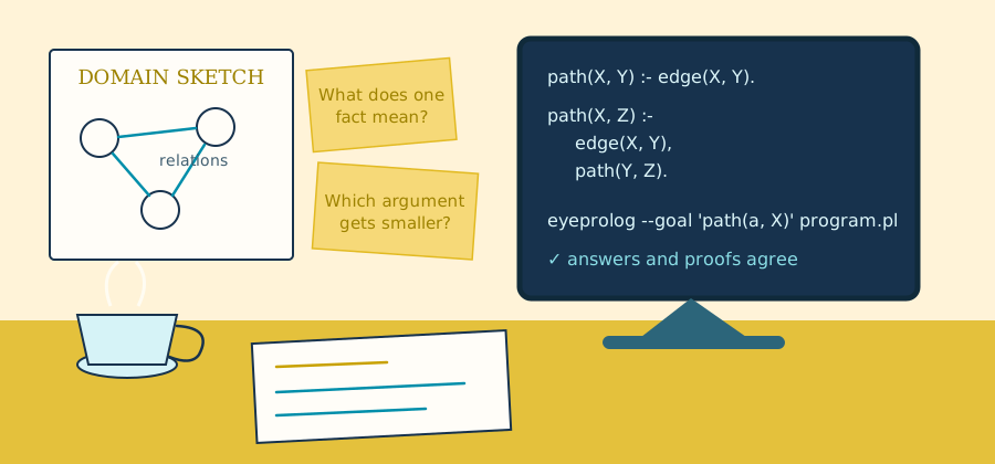
This Part turns from implementation features to habits of construction. A good program rarely arrives whole; it is discovered through examples, corrected by invariants, and refined without losing sight of the relation it is meant to express.
17. Logic and control
The central pleasure—and central difficulty—of logic programming is that a short definition plays two roles. Consider:
:- use_module(library(lists)).

path(X, Y) :- edge(X, Y).
path(X, Z) :- edge(X, Y), path(Y, Z).
As logic, the clauses say that every edge is a path and that an edge followed by a path is a path. As control, they tell the solver to try a direct edge first, then choose an outgoing edge and continue from its endpoint.
This distinction is one of logic programming’s oldest and most durable design ideas. The logical component describes admissible answers; the control component determines which consequences are explored, in what order, and with what resource cost. A change in indexing, goal order, or tabling policy should ideally preserve the first while improving the second. In practice, modeful built-ins and incomplete searches mean that programmers must reason about both.
It is useful to write the relation first as a sentence:
path(X, Y)holds when there is a finite sequence of edges fromXtoY.
That sentence is independent of clause order. It is the specification against which examples and counterexamples can be judged. Only then ask procedural questions: which argument will normally be known, which goal generates a finite set, and which recursive call is smaller or already tabled?
The same relation, a different computation
Conjunction is logically commutative, but its textual order guides search. These two rules have the same intended ground consequences:
:- use_module(library(lists)).

adult(Person) :- person(Person), age(Person, Age), (Age >= 18).

adult(Person) :- (Age >= 18), age(Person, Age), person(Person).
The first is executable in the natural open mode because person/1 and
age/2 bind values before >=/2 inspects them. The second asks a comparison
to operate on unbound variables and fails. Logical equivalence therefore does
not imply equivalent behavior for a goal-directed interpreter with modeful
built-ins.
Clause order also gives a search order. Put simple and common proofs where they can be found cheaply, provided doing so does not starve a necessary base case. A recursive clause that calls itself before consuming input is a warning:
:- use_module(library(lists)).

% Poor control: recursion starts before one list cell is exposed.
bad_member(X, List) :- bad_member(X, Rest), (List = [_ | Rest]).
The usual definition exposes the decreasing structure first:
item(X, [X | _]).
item(X, [_ | Rest]) :- item(X, Rest).
Modes are part of the design
A predicate has one logical meaning but may support several useful calling
patterns. append(Prefix, Suffix, Whole) can:
- construct
Wholewhen the first two arguments are known; - remove a known prefix;
- enumerate every split of a known finite list.
It is not a useful generator when all three arguments are free: there are infinitely many lists. Before accepting a predicate design, make a small mode table:
| Call | Intended use | Finite? |
|---|---|---|
append(+,+,-) |
concatenate | yes |
append(-,-,+) |
enumerate splits | yes |
append(-,-,-) |
generate all triples | no |
The + and - marks are documentation, not supported Prolog syntax.
A mode is a promise about calls, not a replacement for the relation’s meaning. When a rule calls a helper outside its promised mode, the program may remain logically plausible while becoming operationally useless.
Search trees and proof trees
A proof tree contains only the successful choices supporting one answer. A search tree also contains failed alternatives and repeated attempts. Proof output shows the former; performance counters give clues about the latter. Confusing the two leads to a common surprise: a tiny proof may have required a large search.
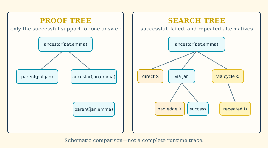
The distinction also explains why explanations are not performance profiles.
Removing a failed branch can make a program dramatically faster without
changing the final why/2 term. Conversely, introducing a well-named helper
may make a proof longer on paper while making it far clearer to a reader.
When a program is slow, sketch the first few levels of its search tree. Mark:
- the selected leftmost goal;
- the clauses or built-ins that can solve it;
- bindings produced by each choice;
- the next selected goal;
- branches that repeat a previous call.
This exercise often reveals that the model is sound but a generator is too broad, a constraint is too late, or a witness carries needless alternatives.
Checkpoint. Take one clause and write two notes beside it: its ground meaning and its intended mode. Reorder two body goals, predict whether the answer set, termination, first answer, or proof shape changes, and only then run the variant.
18. Constructing a program
A good logic program is rarely discovered by typing clauses from top to bottom. It is constructed by moving between examples, relations, and invariants.
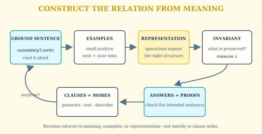
Begin with ground sentences
Suppose packages must be routed through compatible hubs. Start with sentences that contain no variables:
:- use_module(library(lists)).

routeable(parcel_7, hub_north).
Decide exactly what that sentence claims. Does it mean the parcel can enter the hub, can leave it, or can complete an entire route through it? Ambiguity in a ground sentence becomes ambiguity in every rule built on it.
Now name the evidence:
:- use_module(library(lists)).

routeable(Parcel, Hub) :-
  destination_zone(Parcel, Zone),
  serves(Hub, Zone),
  package_class(Parcel, Class),
  accepts(Hub, Class).
The variables express the joins already present in the English explanation. No variable should appear merely because “a value might be needed later.” Every repeated variable asserts identity; every distinct variable permits difference.
Invent examples before recursion
For a recursive relation, write the smallest positive example, the next larger positive example, and a near miss. For list prefixes:
prefix([], [a,b])          true
prefix([a], [a,b])         true
prefix([b], [a,b])         false
The empty example suggests the base clause. Comparing the second example with a smaller one suggests removing a matching head from both lists:
prefix([], _).
prefix([X | Xs], [X | Ys]) :- prefix(Xs, Ys).
This is a general construction method: find a measure that becomes smaller, preserve the invariant while reducing it, and state directly the case where no reduction is needed.
Separate generate, test, and describe
Finite combinatorial programs become easier to read when their jobs are separate:
candidate_pair(A, B) :-
  person(A),
  person(B).

compatible_pair(A, B) :-
  candidate_pair(A, B),
  (A \= B),
  \+ conflict(A, B).

answer(pair(A, B)) :- compatible_pair(A, B).
candidate_pair/2 states the domain. compatible_pair/2 states the
constraints. answer/1 controls presentation. The split is not bureaucratic:
it makes the closed domain visible, gives negation bound arguments, and makes
proofs say whether a step generated or rejected a choice.
For performance, tests may be interleaved as soon as their inputs are ready:
compatible_pair(A, B) :-
  person(A),
  person(B),
  (A \= B),
  \+ conflict(A, B).
The conceptual separation remains even when the final clause is compact.
Choose representations by the operations they support
The same domain can be represented in many ways. A graph may be edge facts, a list of edge terms, or a context. Ask which questions dominate:
- Separate
edge/2facts suit indexed relational lookup and proof provenance. - A list suits passing a private, changing graph through a recursive helper.
- A compound state term suits transitions that replace several components.
- A comma context suits inspecting a small record whose fields are themselves structured assertions.
Do not encode structure into strings and then recover it throughout the
theory. Parse once at the boundary. A term such as
address(City, PostalCode) can be unified, inspected, and explained; a string
containing the same data needs repeated procedural parsing.
Grow a theory through layers
Large rule sets benefit from a dependency direction:
source facts → normalized facts → domain concepts → decisions → answers
Negation should normally point in the same direction, from a higher layer to a complete lower layer. Cycles among positive domain concepts may be tabled; cycles through negation usually signal that the concepts have not been given a stable meaning.
At every layer, add one representative query. Do not wait for the final decision predicate to discover that normalization silently failed. Small queries are the logic-programming counterpart of inspecting intermediate values, but they retain the declarative vocabulary of the model.
Checkpoint. Before writing rules for a small domain of your own, record three positive ground examples, one near miss, the intended query mode, and a candidate finite generator. If the ground sentences are ambiguous, revise the predicate names before introducing variables.
19. Correctness and termination
Testing examples is necessary, but a reusable relation deserves a stronger argument. Two questions should be asked separately:
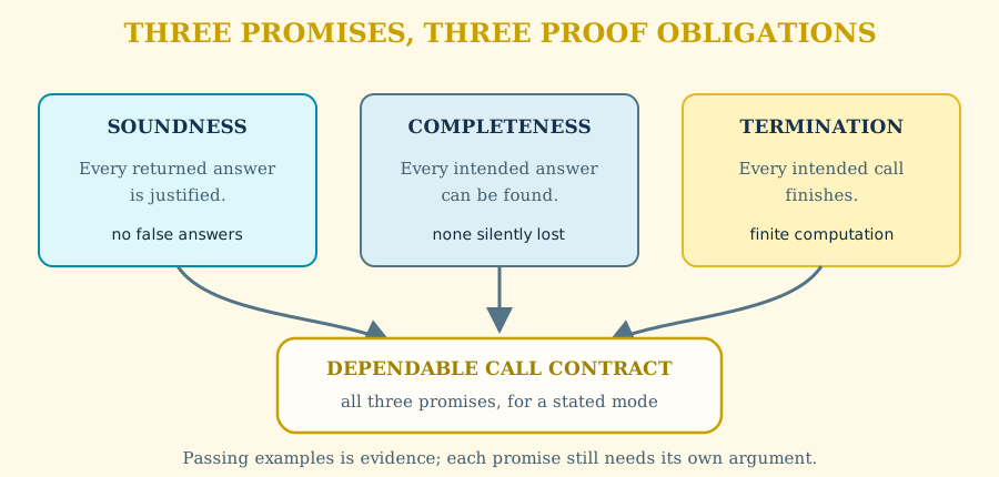
- Partial correctness: if the program returns an answer, is it justified?
- Completeness: for the intended finite calls, can it find every answer required by the specification?
For prefix/2, partial correctness follows from the clauses by induction. The base clause
returns only the empty prefix. The recursive clause adds the same head to a
smaller valid prefix, so the result remains a prefix. Completeness follows in
the opposite direction: every nonempty prefix shares its first element with
the whole list, and removing that element yields a smaller prefix problem
covered by the recursive clause.
This informal induction is often enough. State the property, justify each base clause, assume recursive calls satisfy it, and show that each recursive clause preserves it.
Termination needs its own argument
A correct relation may still fail to return. For ordinary structural recursion, identify a well-founded measure:
- length of the remaining list;
- a nonnegative integer that decreases;
- number of unvisited states in a finite graph;
- size of a syntax tree.
The measure must decrease before the recursive call in the intended mode. For
factorial, N decreases while remaining a nonnegative integer:
factorial(0, 1).
factorial(N, F) :-
  (N > 0),
  (Previous is N - 1),
  factorial(Previous, PF),
  (F is N * PF).
Reordering the subtraction after the recursive call preserves a mathematical equation but destroys the termination argument.
Tabling changes the argument for graph recursion. A cyclic path/2 call can
terminate when the program has only finitely many distinct tabled calls and
answers. The measure is then not necessarily smaller at each edge; finiteness
comes from exhausting a finite answer space. Tabling cannot rescue a rule that
constructs s(s(s(...))) without bound.
Negation and aggregation require bounded subsearch
\+ Goal and aggregates ask the engine to settle a nested search. Their
meaning is usable only when that search can finish. Before
writing:
\+ disqualified(Person)
check that Person is bound and that disqualified/1 has a finite search for
that value. Before collecting routes, decide whether only simple routes, only
routes below a cost, or some other finite family is intended.
Integrity is not merely failure
Ordinary failure says that one attempted proof did not work. An explicit integrity relation can instead return the evidence for an invalid state:
invalid_limits(Name, Low, High) :-
  lower_limit(Name, Low),
  upper_limit(Name, High),
  (Low > High).
This distinction matters operationally and socially. A failed eligibility
query may be a legitimate negative result. A successful invalid_limits/3
query identifies contradictory limits; the host can then stop decisions until
the input is repaired.
Checkpoint. For one recursive relation, state three claims separately: partial correctness, completeness in one intended mode, and termination in that mode. Give the invariant supporting the first two and the decreasing measure or finite table supporting the third.
20. Improving a program
Program improvement begins with observation, not cleverness. Preserve a set of representative answers and proofs, collect solver statistics, and change one structural choice at a time.
Strengthen calls before adding machinery
The most effective improvement is often a better question. Prefer
route(brussels, Destination) to a completely open enumeration if the
application already knows its origin. Put selective, indexed relations early
enough to bind arguments for later work. Avoid constructing a large witness
when the caller needs only existence.
Compare:
connected(X, Y) :- path_with_nodes(X, Y, _).
with a direct reachability relation that tables pairs. The first may enumerate many distinct paths to establish one fact; the second records the fact itself. Keep the witness-producing relation for callers that truly need a path.
Introduce helpers that express invariants
Inlining every condition creates wide clauses with repeated work. A helper can name a stable concept:
within_thermal_limits(Battery) :-
  temperature(Battery, T),
  temperature_limit(Max),
  (T =< Max).
The gain is not just reuse. Proofs now contain a domain statement, and later
changes to the limit policy have one home. Choose helpers that add vocabulary;
avoid names such as step2/3 that merely expose an implementation sequence.
Move invariant work outward
If a recursive call repeatedly computes a value that does not change, compute it once and pass the result:
search(Request, Answer) :-
  normalized_request(Request, Normalized),
  search_normalized(Normalized, initial_state, Answer).
This resembles loop-invariant code motion in procedural programming, but the relational formulation is explicit: the helper’s arguments show exactly which values vary from step to step.
Preserve meaning while changing control
Reordering goals, adding a helper, or specializing a predicate should preserve the intended ground answers. Verify that with:
- ordinary positive examples;
- cases expected to fail;
- duplicate derivations;
- boundary numeric values;
- cyclic data;
- proof premises, not only printed conclusions.
An optimization that changes which proof is found first may affect once/1,
tie-breaking aggregates, and explanation shape even when the answer set is
unchanged. Treat those observable choices as part of the calling contract
whenever users depend on them.
Know when to stop
Not every relation should be made maximally general. A three-mode predicate can be harder to terminate, explain, and index than two simple predicates with clear contracts. Generalize when a real second use appears. The art lies in keeping the logical idea visible while giving it enough control to run well.
Checkpoint. Save representative answers, one proof, and solver statistics for a program. Make exactly one control change, rerun all three views, and classify every difference as intended, harmless but observable, or a regression.
Part IV summary
Part IV treated logic programming as a discipline of construction:
- write the relation’s sentence before choosing its control;
- record intended modes and finite uses;
- begin with ground examples and invent recursion from one proof;
- choose representations by the operations and invariants they expose;
- argue correctness, completeness, and termination separately;
- improve programs by strengthening calls and naming invariants;
- preserve answers while reviewing observable proof or ordering changes.
You should now be able to construct a theory from examples, state a termination measure, refactor a helper without losing meaning, and recognize when greater relational generality has no practical use.
Historical note: logic plus control
Kowalski’s 1979 formulation “algorithm = logic + control” gave a durable name to the dual reading developed here. The logic component specifies knowledge; control determines how it is used. The slogan did not claim that control was unimportant. It argued that control can often be improved while meaning stays steady, and that programs become easier to reason about when the two are distinguished.
The craft tradition of Prolog grew around this tension. Goal ordering, accumulators, generate-and-test, and representation change were never merely interpreter tricks. At their best they were transformations justified by invariants and modes. Sterling and Shapiro made construction and improvement central to The Art of Prolog, showing that declarative clarity and procedural competence mature together.
EyeProlog keeps ISO cut, but Chapter 34 disciplines it: it commits only within
the clause that contains it, never across a disjunction branch or a
meta-call’s own boundary, and it is presented as a last resort next to
once/1 and if-then-else. That discipline changes the techniques but not the
problem: authors must still turn a true relation into a productive computation
and say what was preserved.
Part V — Advanced relational design
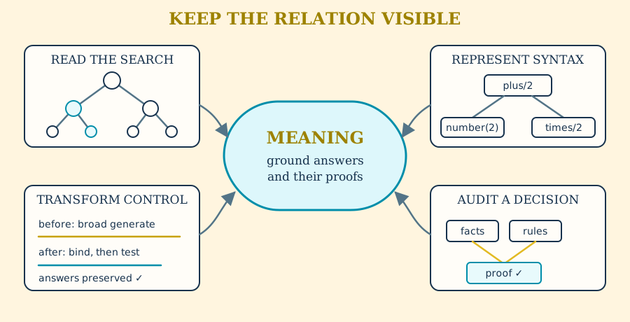
The earlier parts introduced the supported Prolog profile and the habits needed to use it safely. This part stays longer with whole computations. It asks how to inspect a search tree, represent languages and evaluators as relations, transform a correct program without losing its meaning, and organize a decision system whose conclusions remain auditable.
EyeProlog supplies the Part 1 control, dynamic-database, operator, and I/O
facilities together with its normal-profile module forms module/2,
use_module/1, use_module/2, meta_predicate/1, and Module:Goal. The
requirements clarified by the 2013 ISO/IEC 13211-2 module amendment are covered
by a dedicated release-gated suite, including public imports through
ensure_loaded/1 and caller-module qualification of : meta-arguments. The
unchanged remainder of Part 2 is still treated as a compatibility surface, not
as a claim of complete ISO/IEC 13211-2:2000 conformance. Definite-clause grammar notation is
also part of the normal profile, though the running examples have avoided it so far;
Chapter 22 introduces it explicitly rather than assuming it. The examples still prefer
explicit domain relations, state, and syntax trees where that makes assumptions easier to
inspect.
21. Reading the computation
A query is not solved in one leap. It is reduced to goals, each goal is matched against candidate clauses, and each successful match contributes bindings and new subgoals. The computation has two kinds of branching:
- an and step, because every goal in a rule body must succeed;
- an or step, because any matching clause may establish a goal.
This and–or structure is the operational counterpart of the program’s logical structure. A conjunction asks for several supporting claims; multiple clauses offer alternative justifications.
parent(ada, byron).
parent(byron, clara).
parent(clara, diego).

ancestor(X, Y) :- parent(X, Y).
ancestor(X, Z) :- parent(X, Y), ancestor(Y, Z).
eyeprolog --goal 'ancestor(ada, Who)' program.pl
For ancestor(ada, Who), the first clause asks
parent(ada, Who) and produces Who = byron. The second clause asks two
questions in sequence. parent(ada, Y) first binds Y = byron; the remaining
call is therefore ancestor(byron, Who). That call repeats the choice between
a direct-parent proof and a longer proof.
The three answers occupy increasing depths of one proof family:
ancestor(ada, byron)
  parent(ada, byron)

ancestor(ada, clara)
  parent(ada, byron)
  ancestor(byron, clara)
    parent(byron, clara)

ancestor(ada, diego)
  parent(ada, byron)
  ancestor(byron, diego)
    parent(byron, clara)
    ancestor(clara, diego)
      parent(clara, diego)
Drawing even a partial tree exposes errors that are hard to see in source alone: a variable that should have been shared, a recursive call that did not consume input, or a generator placed after the test that needs its output.
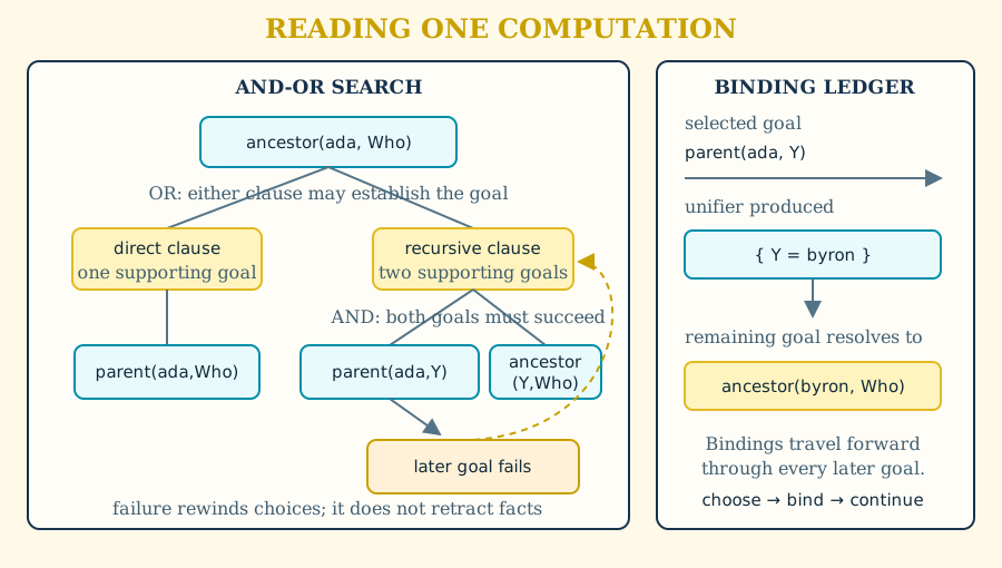
Substitutions accumulate
A substitution is a set of bindings carried through the remaining goals. Bindings are not local return values. If the first goal binds a variable, every later occurrence of that variable sees the same term:
grandparent(X, Z) :-
  parent(X, Y),
  parent(Y, Z).
Solving grandparent(ada, Z) begins with parent(ada, Y). Once that goal
binds Y to byron, the second goal is the selective
parent(byron, Z).
Repeated variables impose equality through unification:
:- use_module(library(lists)).

loop_edge(Node) :- edge(Node, Node).
This does not find an arbitrary edge and compare its endpoints later. The shared variable makes equal endpoints part of the pattern being matched.
Failure rewinds choices, not facts
Suppose a later goal fails:
:- use_module(library(lists)).

eligible(Person) :-
  applicant(Person),
  age(Person, Age),
  (Age >= 18),
  verified(Person).
Failure of verified(Person) rejects the current combination of bindings.
Search may return to another age/2 fact or another applicant clause. It does
not retract source facts or erase answers already printed. Backtracking is
better understood as exploring alternatives than as undoing the world.
Variants, cycles, and tables
Recursive graph search can encounter the same logical subquestion through
different paths. Calls that differ only in variable names are variants:
path(a, X) and path(a, Y) pose the same pattern. Positive recursive groups
can table such patterns, share their answers, and stop a cycle from expanding
the same question forever.
The table does not prove termination for every recursive program. If each call constructs a larger pattern, then the calls are not variants:
grows(X) :- grows(wrapper(X)).
grows(A), grows(wrapper(A)), and
grows(wrapper(wrapper(A))) are distinct calls. Remembering them does not
make their number finite.
A practical tracing discipline
When a query surprises you, write down:
- the selected goal;
- its current resolved arguments;
- the candidate clause;
- the unifier produced by the head;
- the new body goals;
- the point to which failure would return.
Compare that hand trace with --proof for a successful answer and --stats
for the amount of search. Proofs explain one successful derivation; statistics
summarize work across successful and failed branches. Neither is a complete
trace, but together they usually locate the modeling issue.
Exercises.
- Draw the and–or tree for
ancestor(byron, Who). - Add a second parent of
claraand identify where the tree branches. - Write a cyclic
edge/2graph and compare reachability answers with the table rounds reported by--stats. - Construct a recursive rule whose call grows a list on every step. Explain why variant tabling does not make its call space finite.
Checkpoint. Hand-trace one successful answer and one failed branch using
the six-item tracing discipline. Compare the successful trace with --proof
and the total work with --stats; state one fact that each view omits.
22. Trees, languages, and symbolic evaluation
Compound terms are finite trees. A functor labels an internal node and its arguments are the children. Lists are one familiar tree encoding, but syntax, plans, types, circuits, formulas, and organizational structures can all be represented directly.
tree(
  oak,
  tree(birch, empty, empty),
  tree(pine, empty, empty)
).
A structural relation follows the representation:
:- use_module(library(lists)).

tree_member(X, tree(X, _, _)).
tree_member(X, tree(_, Left, _)) :- tree_member(X, Left).
tree_member(X, tree(_, _, Right)) :- tree_member(X, Right).
The clauses say where a member may occur. They also define a search order:
root, then left subtree, then right subtree. If only membership matters, that
order is an implementation choice. If a caller uses once/1, it becomes
observable.
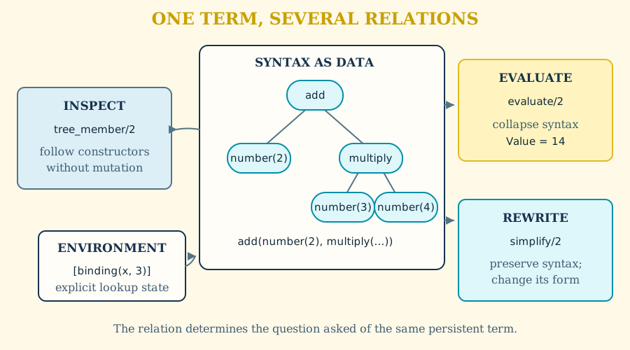
Transforming a tree
mirror(empty, empty).
mirror(
  tree(Value, Left, Right),
  tree(Value, MirroredRight, MirroredLeft)
) :-
  mirror(Left, MirroredLeft),
  mirror(Right, MirroredRight).
Read forward, mirror/2 constructs a mirror. With both trees ground, it
verifies the relationship. In some partially bound modes it can fill missing
structure. The rule does not mutate a tree; it relates two persistent terms.
The representation exposes an invariant: mirroring preserves every node value and exchanges left and right at every level. It also suggests a structural induction. The empty tree is its own mirror; if both recursive calls are correct, the constructed parent is correct.
A standard definite clause grammar
ISO/IEC TS 13211-3 definite clause grammar rules describe a sequence while the processor supplies the pair of difference-list arguments used for execution:
sentence --> noun_phrase, verb_phrase.

noun_phrase --> [the], noun.
noun_phrase --> [a], noun.

noun --> [robot].
noun --> [scientist].

verb_phrase --> verb, noun_phrase.

verb --> [helps].
verb --> [observes].

complete_sentence(Words) :- phrase(sentence, Words).
eyeprolog --goal 'complete_sentence([the, robot, helps, a, scientist])' program.pl
The expansion of sentence//0 is an ordinary sentence/2 relation: its first
extra argument is the sequence before parsing and its second is the suffix.
Composition shares the suffix from noun_phrase//0 with the input to
verb_phrase//0. phrase/2 requires complete consumption; phrase/3 exposes
the remaining sequence.
The same relation can be a bounded generator when vocabulary and output length
are constrained by surrounding relations. An unconstrained
complete_sentence(Words) call can generate sentences of unbounded length if
the grammar is recursive. A grammar is also a search program, so its intended
modes need the same termination analysis as other recursive relations.
Interpreting an expression
Syntax trees separate the expression from the act of evaluating it:
evaluate(number(N), N).

evaluate(add(Left, Right), Value) :-
  evaluate(Left, L),
  evaluate(Right, R),
  (Value is L + R).

evaluate(multiply(Left, Right), Value) :-
  evaluate(Left, L),
  evaluate(Right, R),
  (Value is L * R).
eyeprolog --goal 'evaluate(
    add(number(2), multiply(number(3), number(4))),
    Value
  )' program.pl
The value is 14. More importantly, the proof follows the syntax tree: two
literal evaluations support one multiplication and one addition.
An extension can add variables and an explicit environment:
:- use_module(library(lists)).

lookup(Name, [binding(Name, Value) | _], Value).
lookup(Name, [_ | Rest], Value) :- lookup(Name, Rest, Value).

evaluate(variable(Name), Environment, Value) :-
  lookup(Name, Environment, Value).
Passing the environment as data avoids hidden global state. Shadowing is
determined by list order and should be documented as part of lookup/3.
Rewriting symbolic expressions
Evaluation collapses syntax to a value. Rewriting preserves syntax while replacing one form with an equivalent or preferred form:
simplify(add(number(0), X), X).
simplify(add(X, number(0)), X).
simplify(multiply(number(1), X), X).
simplify(multiply(X, number(1)), X).

simplify(add(A, B), add(SA, SB)) :-
  simplify(A, SA),
  simplify(B, SB).
Overlapping rules can produce several answers. That may be desirable when
exploring equivalent forms, but a normalizer needs a strategy and termination
measure. A rule that expands X to add(X, number(0)) reverses the first
simplification and permits unbounded rewriting.
Exercises.
- Define
tree_size/2andtree_height/2. - Extend the grammar with adjectives while preserving the input/suffix contract.
- Add subtraction to the evaluator and state which arguments must be ground.
- Define constant folding for
add(number(A), number(B)). - Explain why individually sensible rewrite rules may fail to terminate when repeatedly combined.
Checkpoint. For one compound term, label the object-language syntax, the EyeProlog relation that inspects it, and the environment or state used to interpret it. Then identify a rewrite pair that would create a cycle if both directions were enabled.
23. Transforming programs
Program transformation changes clauses while attempting to preserve an intended relation. The useful question is not merely “does the new version run?” but “for which calls does it preserve answers, termination, answer order, and explanations?”
Four transformations recur in logic programs:
- unfolding replaces a call by the bodies of its defining clauses;
- folding names a repeated conjunction with a helper relation;
- specialization fixes known arguments and removes irrelevant choices;
- accumulation carries a partial result through recursion.
Each can improve control or reveal structure. Each can also change modes, duplicate work, or alter proof shape.
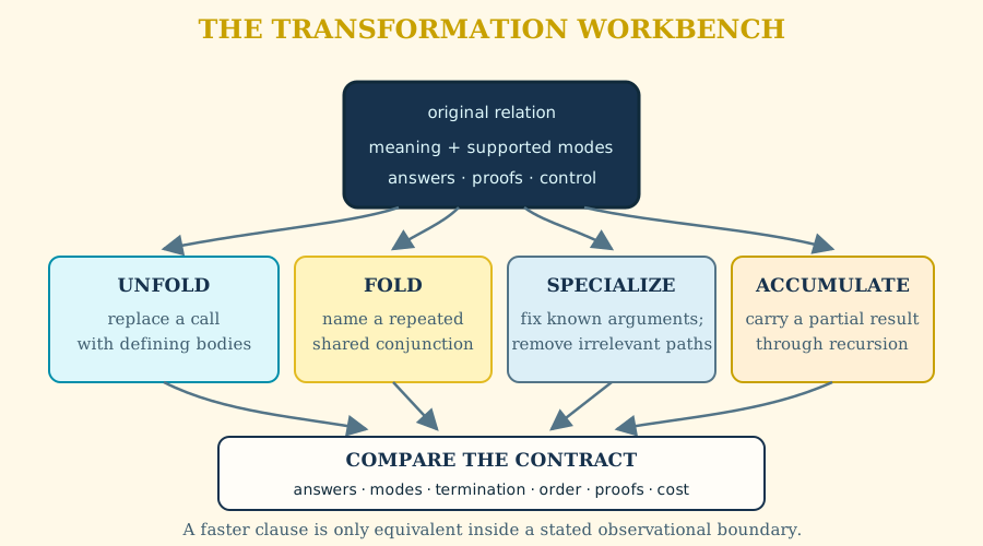
Unfolding and folding
Start with:
:- use_module(library(lists)).

adult(Person) :-
  recorded_age(Person, Age),
  adult_age(Age).

adult_age(Age) :- (Age >= 18).
Unfolding adult_age/1 gives:
:- use_module(library(lists)).

adult(Person) :-
  recorded_age(Person, Age),
  (Age >= 18).
For this deterministic helper, the ground answers are unchanged. The shorter
proof loses the named concept adult_age/1, however. That loss may be
undesirable in an auditable policy even if execution becomes slightly cheaper.
If a helper has several clauses, unfolding produces one caller clause for each
alternative. If it is recursive, unrestricted unfolding may never finish.
Folding moves in the other direction. Suppose decisions repeat:
:- use_module(library(lists)).

can_board(Person) :-
  registered(Person),
  identity_checked(Person),
  \+ suspended(Person),
  has_ticket(Person).

can_enter_lounge(Person) :-
  registered(Person),
  identity_checked(Person),
  \+ suspended(Person),
  lounge_pass(Person).
Name the shared concept:
:- use_module(library(lists)).

traveler_in_good_standing(Person) :-
  registered(Person),
  identity_checked(Person),
  \+ suspended(Person).

can_board(Person) :-
  traveler_in_good_standing(Person),
  has_ticket(Person).

can_enter_lounge(Person) :-
  traveler_in_good_standing(Person),
  lounge_pass(Person).
The helper is valuable because it has a stable meaning, not merely because
three lines became one. It creates one place to state and test the closed-world
assumption behind \+ suspended(Person).
Specializing a relation
A general transport database may use:
connection(Mode, From, To, Cost).
An application that only plans rail journeys can define:
rail_connection(From, To, Cost) :-
  connection(rail, From, To, Cost).
This wrapper establishes a stronger contract and gives indexing a bound first argument. Deeper specialization can precompute invariant classifications or remove irrelevant branches. Keep the general relation as the specification against which specialized answers are compared.
Accumulators and modes
A direct list sum performs work after recursion:
sum_numbers([], 0).
sum_numbers([X | Xs], Sum) :-
  sum_numbers(Xs, Rest),
  (Sum is X + Rest).
An accumulator makes the partial sum explicit:
sum_numbers_acc(List, Sum) :- sum_from(List, 0, Sum).

sum_from([], Accumulator, Accumulator).
sum_from([X | Xs], Accumulator, Sum) :-
  (Next is Accumulator + X),
  sum_from(Xs, Next, Sum).
For a ground numeric list, both versions return the same sum. They do not have identical relational behavior in every mode. The accumulator version requires each intermediate addition to be ready on the way down. State the intended mode instead of claiming unconditional equivalence.
A transformation checklist
Before replacing one definition with another, record:
- the intended ground relation;
- supported binding patterns;
- a termination measure for each supported pattern;
- whether duplicates and answer order matter;
- whether callers inspect proof structure;
- representative positive, negative, and boundary queries.
Then compare both versions. --stats can show fewer calls or unifications, but
performance evidence comes after semantic evidence. A faster program that
silently drops a mode is a different program. Predicate and inference counts are
also not reliable substitutes for elapsed time: one expensive host call can cost
more than thousands of cheap Prolog calls. Repository-level performance work
watches npm test’s own elapsed time across the whole corpus rather than a
dedicated wall-clock benchmark harness.
Exercises.
- Unfold a two-clause helper and count the resulting caller clauses.
- Fold repeated validation conditions in two rules of your own.
- Specialize a generic graph relation for one edge type.
- Compare direct and accumulator-based length relations in several modes.
- Find a transformation that preserves answers but changes the first proof
selected by
once/1.
Checkpoint. Choose one original and transformed relation. Compare their answer sets in both directions over a finite domain, then separately compare termination, answer order, duplicates, proof shape, and solver statistics.
24. Designing finite search
Nondeterminism is not randomness. A nondeterministic relation defines several legitimate continuations, and search systematically explores them. The design problem is to make useful alternatives complete while keeping their number finite and their order productive.
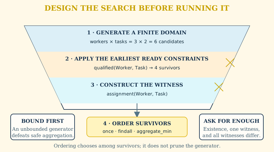
Generate, constrain, describe
A clear search program often has three layers:
- generate a candidate from a finite domain;
- constrain the candidate;
- describe or score the surviving witness.
worker(ada).
worker(byron).
worker(clara).

task(inspect).
task(repair).

qualified(ada, inspect).
qualified(byron, repair).
qualified(clara, inspect).
qualified(clara, repair).

assignment(Worker, Task) :-
  worker(Worker),
  task(Task),
  qualified(Worker, Task).
eyeprolog --goal 'assignment(Worker, Task)' program.pl
worker/1 and task/1 make the search space explicit. qualified/2 is both a
constraint and a selective relation. If the application knows the task,
calling assignment(Worker, repair) avoids generating irrelevant task values.
Search over states
A state-space problem needs a state term, a finite move relation, a goal test, a policy for repeated states, and a witness representation. A simple graph path carries visited nodes:
:- use_module(library(lists)).

simple_path(From, To, Path) :-
  walk(From, To, [From], Reversed),
  reverse(Reversed, Path).

walk(To, To, Visited, Visited).
walk(From, To, Visited, Path) :-
  edge(From, Next),
  \+ member(Next, Visited),
  walk(Next, To, [Next | Visited], Path).
The visited list makes the witness finite on a finite graph. It also changes the question from arbitrary walks to simple paths. That is a modeling choice, not merely an optimization. A caller asking for repeated stops needs another bound, such as maximum steps or cost.
Existence, one witness, and all witnesses
These questions have very different costs:
:- use_module(library(lists)).

reachable(From, To).
once(simple_path(From, To, Path)).
findall(Path, simple_path(From, To, Path), Paths).
Reachability needs only a pair and is a good candidate for tabling. One path may stop after the first witness. All simple paths may be exponentially numerous even though the graph is finite. Choose the weakest result that meets the caller’s need.
Optimization is search plus an order
An optimal answer requires a finite candidate relation and a comparison key:
:- use_module(library(aggregate)).
:- use_module(library(lists)).

best_plan(Request, Plan, Cost) :-
  aggregate_min(
    [CandidateCost, CandidatePlan],
    CandidatePlan,
    candidate_plan(Request, CandidatePlan, CandidateCost),
    [Cost, Plan],
    Plan
  ).
The structured key makes ties deterministic. It does not reduce the candidate
space: aggregate_min/5 must settle the nested search before knowing the
minimum. For a large problem, strengthen candidate_plan/3 or use a
domain-specific dynamic program instead of assuming aggregation performs
branch-and-bound.
Fairness and depth-first search
Depth-first clause search can become trapped in an infinite branch before reaching a later finite proof. Base cases should be reachable before recursive expansion, and recursive steps should consume a finite resource or enter a finite table. When neither is possible, the query is outside the practical contract of the relation.
Multiple clauses normally mean that any or all may yield legitimate answers.
once/1 turns the first success into a don’t-care choice: later alternatives
are intentionally discarded. Use it only when selection order is an accepted
part of the specification.
Exercises.
- Add skills and time slots to the assignment example.
- Modify
simple_path/3to return accumulated cost. - Compare reachability, one path, and all paths on a diamond-shaped graph.
- Give a finite candidate relation for which
aggregate_min/5still performs an impractically large search. - Construct a recursive first clause that starves a valid later base clause, then repair its control.
Checkpoint. Write down the size of a candidate space before running its search. Name the generator, the earliest ready constraint, the witness, and the ordering used for optimization. If the size cannot be bounded, the design is not yet ready for aggregation.
25. Case study: an auditable decision service
This case study develops a small access decision from prose to an executable, explainable theory. The purpose is the sequence of design decisions that turns informal requirements into maintainable relations.
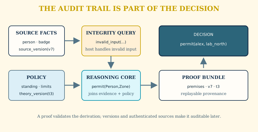
Requirements and questions
A research facility says:
- a person may enter a zone when their badge is active;
- the badge must grant the zone’s required clearance;
- required training must be current;
- an explicit suspension blocks entry;
- contradictory badge records invalidate the decision service;
- every permit should carry a reason traceable to source facts.
Before coding, identify ambiguities. Is the badge registry complete? Is missing training evidence a denial or unknown? Can a person have several active badges? Which clock determines “current”? A rule engine cannot remove these choices; it can only make the chosen answers precise.
Source and concept layers
Represent observations without embedding decisions:
:- use_module(library(lists)).

person(ada).
badge(b17, ada).
badge_status(b17, active).
badge_clearance(b17, laboratory).
zone_requires(clean_room, laboratory).
training_valid(ada, clean_room).
The badge identifier remains explicit. Collapsing it into
active_badge(ada) would hide the record used as evidence and make conflicting
records harder to detect.
Build vocabulary that reads like the policy:
:- use_module(library(lists)).

active_badge(Person, Badge) :-
  badge(Badge, Person),
  badge_status(Badge, active).

cleared_for(Badge, Zone) :-
  badge_clearance(Badge, Clearance),
  zone_requires(Zone, Clearance).

prepared_for(Person, Zone) :-
  training_valid(Person, Zone).
Each helper has one responsibility. A proof of cleared_for/2 names both the
badge clearance and zone requirement rather than burying their join in a wide
decision clause.
Closed-world choice
If the suspension list is authoritative and complete, absence can be used:
in_good_standing(Person) :-
  person(Person),
  \+ suspended(Person).
If it is incomplete, this rule is unsound as policy. Replace it with a positive
source claim such as standing(Person, good). The difference is an agreement
about the knowledge boundary, not a matter of syntax.
Decision, reasons, and proof
:- use_module(library(lists)).

permit(Person, Zone) :-
  active_badge(Person, Badge),
  cleared_for(Badge, Zone),
  prepared_for(Person, Zone),
  in_good_standing(Person).

reason(Person, Zone, badge_and_training_verified) :-
  permit(Person, Zone).
eyeprolog --goal 'permit(Person, Zone)' program.pl
eyeprolog --goal 'reason(Person, Zone, Reason)' program.pl
reason/3 supplies a stable user-facing summary. With --proof, the same
answer carries its detailed derivation. These are complementary: the reason is
domain vocabulary, while the proof records actual clauses and bindings.
Integrity before decisions
Contradictory badge states are exposed by an explicit validation relation:
incompatible_status(active, revoked).
incompatible_status(revoked, active).

invalid_badge_status(Badge, Status, Other) :-
  badge_status(Badge, Status),
  incompatible_status(Status, Other),
  badge_status(Badge, Other).
This result does not say that one permit failed. It identifies input that is
unfit for a trusted decision. The host can query invalid_badge_status/3 before
permit goals, alongside checks for a badge assigned to two people or a zone
with incompatible clearance definitions.
Tests are policy examples
A useful test set includes an ordinary permit, missing training, suspension, insufficient clearance, duplicate derivations, contradictory status, and a proof showing the exact badge and training facts.
Boundary examples reveal requirements. If a person has two valid badges,
should there be one permit with two derivations or two permit terms containing
the badge? permit(Person, Zone) chooses one ground decision with potentially
several proofs. If badge identity belongs in the answer, define
permit(Person, Zone, Badge).
Embedding and audit
Authenticate source systems in the host, convert records to EyeProlog facts, run the theory, and store the answer with its proof and input version. The solver can explain logical support; it cannot attest that a badge database was current or a training provider trustworthy.
authenticated source snapshot
  -> normalized EyeProlog facts
  -> checked theory
  -> permit and reason
  -> proof referencing clauses and facts
When policy changes, preserve old inputs, theory versions, and proofs so a past decision can be reconstructed under the rules that actually governed it.
Exercises.
- Add time-bounded training using explicit dates and
difference/3. - Model
denial/3without assuming every failed permit has the same reason. - Add a two-person escort rule and identify duplicate-proof cases.
- Write an integrity relation for badges assigned to multiple people.
- Define the validation the host must perform before supplying badge facts.
- Run the case with
--proofand decide which helpers improve the explanation.
Checkpoint. Reconstruct one permit decision from a preserved source snapshot, theory version, answer, and proof. Mark which step authenticates the source, which checks integrity, which derives the decision, and which merely stores evidence for later audit.
Part V summary
Part V followed whole computations rather than isolated features:
- and–or trees expose conjunction, alternatives, failure, and repeated calls;
- explicit syntax trees support grammars, evaluators, and symbolic rewriting;
- unfolding, folding, specialization, and accumulators transform control under stated invariants;
- finite search needs a declared space, pruning argument, witness, and fairness expectation;
- an auditable service layers sources, concepts, integrity, decisions, reasons, embedding, and proof retention.
You should now be able to trace substitutions through several goals, represent an object language without confusing it with the surrounding Prolog syntax, justify a bounded program transformation, and design a reconstructable decision theory.
Historical note: interpreters, transformation, and the art tradition
Logic programming became a laboratory for symbolic programming because its principal data—terms, clauses, substitutions, and proof trees—could be represented with the same structures used for ordinary domains. Meta-interpreters made resolution itself a program topic; grammar rules made language recognition relational; partial evaluation showed how a general relation could be specialized when part of its input was known.
Futamura’s work in the 1970s gave partial evaluation a striking interpretation: specializing an interpreter with respect to a source program can produce a compiled form. Logic-program transformation developed related practices of unfolding, folding, and specialization. The inheritance for EyeProlog is not a promise that every classic transformation is built in. It is the demand that a transformation name its invariant and preserve a stated answer contract.
The Art of Prolog joined computation, construction, nondeterminism, grammars, interpreters, transformation, and applications into a sustained account of craft. Part V pays tribute to that breadth through EyeProlog’s explicit subset: syntax is data, state is an argument, and audit evidence remains visible.
Part VI — Mathematics made executable
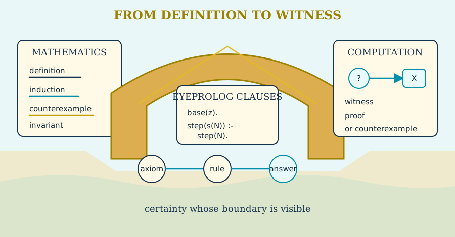
This Part is a route, not a prerequisite for the reasoning laboratory. For a short practical path, read Chapters 26, 27, and 29, then continue at Chapter
- Read Chapters 28 and 30 as well when representation, formal scope, and the limits of computation are central to your purpose.
Mathematics appears throughout this book as subject matter: arithmetic, combinatorics, graphs, geometry, algebra, statistics, and physical models. But its deeper presence is structural. A logic program is possible because parts of mathematical reasoning can be represented as finite symbols, transformed by explicit rules, and checked step by step.
In that qualified sense, the history of logic programming belongs inside the history of mathematics. It inherits the mathematician’s old practices of definition, proof, construction, abstraction, and counterexample. It also inherits the twentieth century’s harder questions. What counts as a formal proof? What is an effective procedure? Which truths follow from a finite set of axioms? Which questions cannot be decided by any uniform mechanical method?
EyeProlog inherits a small, practical fragment of that tradition. It is not a foundation for all mathematics, a computer algebra system, or an interactive theorem prover. Its definite clauses cover only a disciplined fragment of logic. Precisely because the fragment is small, however, one can see the ancient mathematical acts inside the running machine:
| Mathematical act | EyeProlog form | Operational consequence |
|---|---|---|
| Define a class | facts and clauses | enumerate its instances |
| Introduce an unknown | a variable | seek a substitution |
| Use a lemma | call a helper relation | open a subgoal |
| Split into cases | multiple clauses | create alternatives |
| Perform induction | base and recursive clauses | reduce to smaller calls |
| Construct a witness | bind an output term | return evidence, not only truth |
| Refute a universal guess | search for a counterexample | one answer is enough |
| Check consistency | an explicit integrity query | reject or report invalid input |
| Explain a conclusion | a proof term | expose the successful derivation |
The table is a correspondence, not an identity. A mathematical proof and an EyeProlog execution answer different questions unless the encoding between them is itself justified. This Part develops both the power and the limit of the correspondence.
26. A proof can be a computation
For most of mathematical history, an algorithm and a proof could live close together without being regarded as the same kind of object. Euclid’s algorithm computes a greatest common divisor, while Euclid’s propositions justify why the procedure works. A geometrical construction produces an object, while an argument establishes that it has the required properties. The distinction remains useful, but modern logic revealed increasingly exact connections among a proposition, its proof, and the construction carried by that proof.
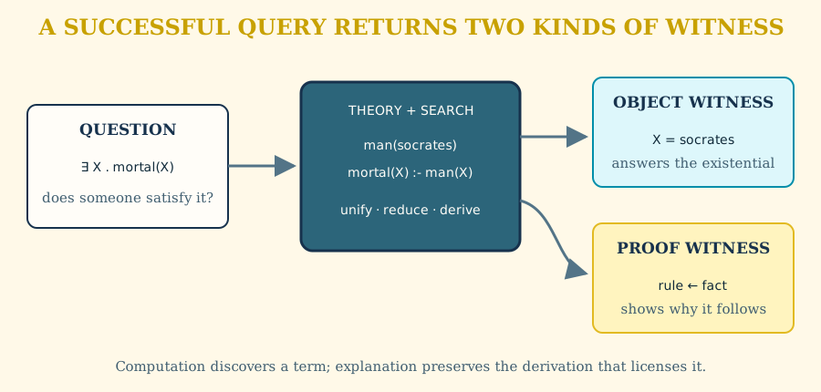
Logic programming enters through one particular connection. A definite clause
mortal(X) :- human(X).
is at once an implication-like statement and an instruction for reducing the
question mortal(socrates) to the subquestion human(socrates). A successful
derivation does not merely return true; it records a sequence of justified
reductions and the substitutions that made them fit.
From axioms to effective procedure
The route was neither straight nor inevitable. A compact historical spine is:
- Axiomatization. Nineteenth- and early-twentieth-century mathematics sharpened the demand that assumptions and inference rules be stated explicitly. Hilbert’s program made formal proof and consistency central mathematical subjects.
- Limits of formal systems. Gödel showed that sufficiently expressive, effectively axiomatized consistent systems cannot capture every arithmetical truth within themselves. Formalization acquired proven limits, not merely engineering difficulties.
- Effective calculability. Church and Turing gave exact, extensionally equivalent accounts of effective computation and established that some decision problems have no general algorithm.
- Ground instances. Herbrand connected quantified first-order statements to finite combinations of ground instances. The terms used to instantiate variables became central proof objects.
- Machine-oriented inference. Robinson’s resolution principle combined clauses and unification into a small general proof mechanism.
- Logic as a programming language. Prolog specialized these ideas into an executable discipline, and the least-model and fixed-point semantics of van Emden and Kowalski explained how definite programs denote their ground consequences.
Each step narrowed one ambiguity while uncovering another. Formal syntax made proofs mechanically inspectable, but Gödel marked the boundary of formal completeness. Models of computation made “algorithm” exact, but Church and Turing marked the boundary of decidability. Resolution made inference uniform, but a proof procedure still needed control: selection order, clause order, termination discipline, and eventually tabling.
Logic programming is therefore not the historical triumph of machinery over mathematics. It is one result of mathematics becoming reflective about its own methods.
Answers are existential witnesses
Consider a relation for a Pythagorean triple:
:- use_module(library(between), [between/3]).
:- use_module(library(lists)).

triple(A, B, C) :-
  between(1, 20, A),
  between(A, 20, B),
  between(B, 20, C),
  (AA is A * A),
  (BB is B * B),
  (Sum is AA + BB),
  (Sum is C * C).
eyeprolog --goal 'triple(A, B, C)' program.pl
The open query asks an existential question over a finite domain: find values for which the equation holds. Each printed ground answer is a witness. The substitution is not an incidental side effect; it is the computational content of the existential claim.
A verifier and a generator are logically close but operationally different.
If A, B, and C are already known, the arithmetic goals check a candidate.
If they are unknown, the bounded between/3 calls create candidates first.
The equation alone does not tell a mode-sensitive evaluator where numbers
should come from.
This is an important distinction between mathematical existence and executable witness production. A classical proof may establish that something exists without furnishing an efficient construction. An EyeProlog query produces a witness only when its clauses and control actually reach one.
Proof objects and proof checking
The normal answer
:- use_module(library(lists)).

triple(3, 4, 5).
states the result. Proof output adds the successful chain of facts, rule uses, built-ins, and bindings. That evidence supports three different activities:
- rechecking: verify that every step follows from the supplied theory and built-in contract;
- auditing: identify which premises were actually used;
- explanation: translate a derivation into domain reasons a person can inspect.
These activities must not be conflated. A derivation can be mechanically valid but pedagogically obscure. It can be clear but depend on an untrustworthy source fact. It can be valid in the implemented arithmetic but fail to express the intended physical quantity. Proof output makes scrutiny possible; it does not perform all scrutiny on the reader’s behalf.
The least model as mathematical closure
For a definite program, begin with its ground facts. Repeatedly add every ground rule head whose ground body is already satisfied. The least fixed point of this operation is the least Herbrand model.
For
:- use_module(library(lists)).

edge(a, b).
edge(b, c).

path(X, Y) :- edge(X, Y).
path(X, Z) :- edge(X, Y), path(Y, Z).
the closure first contains the two edges, then the corresponding direct paths,
then path(a, c). No unsupported path is added. Bottom-up closure and
goal-directed proof search approach the same declarative meaning from opposite
directions: one asks what follows globally, the other asks what is needed for
this goal.
Explicit tabling makes the connection visible. A table for a declared recursive component grows monotonically with newly discovered answers until no rule adds another. The implementation is performing a local, demand-driven fixed-point calculation.
There is an important lifetime distinction between a table that is needed to
finish one fixed point and a cache of tables retained for possible later reuse.
DCG nonterminals are ordinary predicates after expansion, so they are depth-first
unless their expanded predicate indicator is explicitly tabled. Untabled
list-tail DCGs such as ... --> [_], ... therefore run directly with standard
Prolog control. For an explicitly tabled grammar invoked through phrase/2-3,
EyeProlog instead uses a separate invocation-keyed table scope rather than
retaining tables for unrelated input sequences — a declared table remains a
conscious source-level choice.
Exercises.
- Run the triple program with one, two, and three arguments bound. Compare the logical question, answer set, and search size.
- Add a primitive-triple test by rejecting triples whose three values share a divisor. State exactly which finite generators make the negation safe.
- Inspect
examples/fundamental-theorem-arithmetic.pl. Separate the witness it constructs from the property it verifies. - Draw the fixed-point stages for a four-edge graph containing one cycle.
- Find a proof whose machine form is correct but whose helper names make it a poor human explanation.
Checkpoint. For one printed mathematical answer, state the existential claim witnessed by its bindings, the finite domain that made search effective, and the separate argument—if any—that justifies a universal theorem.
27. Recursion is induction in motion
Recursion and mathematical induction are not identical, but they are natural partners. Induction justifies a statement for every object generated by a finite construction. Recursion defines a result by following that same construction toward smaller objects.
For natural numbers represented as z, s(z), s(s(z)), and so on:
natural(z).
natural(s(N)) :- natural(N).

plus(z, Y, Y).
plus(s(X), Y, s(Z)) :- plus(X, Y, Z).
The clauses for plus/3 say:
- adding zero to
YproducesY; - adding the successor of
XtoYproduces the successor of the result of addingXtoY.
Operationally, the first argument decreases by one constructor until it reaches
z. Mathematically, the clauses mirror a recursive definition. To prove a
property of plus/3 for all Peano naturals, induction on that first argument is
the obvious proof shape.
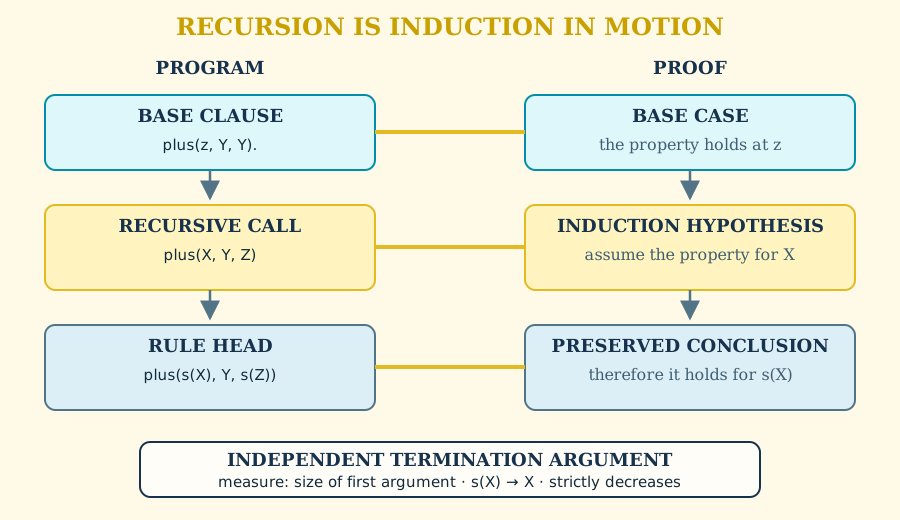
Three obligations, not one
A recursive mathematical program invites three separate arguments:
- Partial correctness: if the relation returns an answer, does the answer satisfy the intended specification?
- Completeness for the intended mode: if an answer satisfies the specification, will this program find it?
- Termination: will search finish for calls in the intended mode?
They are logically independent. A program can terminate and return the wrong answer. It can return only correct answers while missing some. It can describe the correct relation and still diverge before producing it.
For plus(+,+,-), a termination measure is the number of s/1 constructors in
the first argument. Every recursive call strictly decreases that natural
number. The measure is well-founded: there is no infinite descending sequence
of natural numbers.
That last sentence is the mathematical heart of a termination proof. “It seems to get smaller” is not enough. Name a set with no infinite descent, give a measure into that set, and show strict decrease on every recursive branch.
Structural induction and data design
Lists carry their induction principle in their syntax:
- base object:
[]; - constructor:
[Head | Tail].
A relation following that structure is easy to reason about:
:- use_module(library(lists)).

list_length([], 0).
list_length([_ | Tail], N) :-
  list_length(Tail, M),
  (N is M + 1).
To prove that list_length(List, N) returns the number of cells in a finite
proper list, prove the empty case, then assume the claim for Tail and prove
it for [Head | Tail]. The recursive program and inductive proof share a
skeleton because both respect the same constructors.
Representation can either expose or obscure this skeleton. A syntax tree built
from number/1, plus/2, and times/2 supports structural recursion directly.
A flat token string requires parsing before the same argument becomes visible.
Good representations do not merely save code; they make invariants and proof
principles available.
Accumulators and strengthened invariants
An accumulator often improves control but makes the induction hypothesis more subtle:
reverse_acc(List, Reversed) :-
  reverse_go(List, [], Reversed).

reverse_go([], Acc, Acc).
reverse_go([X | Xs], Acc, Reversed) :-
  reverse_go(Xs, [X | Acc], Reversed).
The useful invariant is not merely “Reversed is the reverse of Xs.” It is:
reverse_go(Xs, Acc, Reversed)holds whenReversedis the reverse ofXsplaced beforeAcc.
Strengthening the statement makes the recursive step provable. This is a classic mathematical move: a theorem that is too weak to support induction is generalized until the induction hypothesis contains what the next step needs. Program transformation and proof discovery meet at the invariant.
Tabling changes the termination argument
Ordinary structural recursion terminates by decreasing a term. Graph reachability on a cyclic finite graph has no such simple decrease: following an edge can return to an earlier vertex. Tabling supplies a different well-founded argument.
If the graph has finitely many vertices, then there are finitely many possible
ground path/2 answers. A table only grows; each productive iteration adds a
previously unseen answer; therefore only finitely many productive iterations
are possible. Termination follows from finiteness of the answer space rather
than structural descent of each call.
The proof also states its boundary. If rules construct terms of unbounded depth, the set of possible calls or answers may be infinite, and tabling no longer supplies a finite bound.
Exercises.
- State partial correctness, completeness, and termination claims for
plus(+,+,-)separately. - Define multiplication over Peano naturals and give its decreasing measure.
- Prove the strengthened
reverse_go/3invariant on paper. - Compare the termination arguments for list membership and cyclic graph reachability.
- Study
examples/peano-calculus.pland identify where the data constructors determine the available induction.
Checkpoint. Align one recursive program with an inductive argument: base clause with base case, recursive call with induction hypothesis, and rule head with the preserved conclusion. Then give the independent termination measure.
28. Algebra, symmetry, and representation
Algebra studies operations by the laws they satisfy rather than by the material of the objects being operated on. Logic programming has a similar appetite for structure. Unification ignores the private identity of a variable name and asks whether two terms have a common instance. A relational program often works over lists, trees, graphs, substitutions, or group elements because the clauses depend only on their constructors and laws.
Unification is structural equation solving
The goal
(pair(X, f(Y)) = pair(g(a), f(b))).
decomposes into structural equations. The outer functors and arities agree,
so corresponding arguments must agree; the resulting substitution is
X = g(a) and Y = b.
This resembles algebraic equation solving, but unification is more specific.
It operates in the free term algebra: different constructors are distinct,
and two constructed terms agree only when their outer symbols and corresponding
arguments agree. It does not know, unless clauses or built-ins say so, that
X is 2 + 3 and X is 3 + 2 express a commutative operation.
The distinction prevents a common conceptual error:
- syntactic equality comes from identical term structure or unification;
- domain equality may require mathematical laws, normalization, or a decision procedure.
For polynomials, matrices, groups, or sets, choosing a canonical representation can turn some domain equalities into syntactic equalities. But the normalization algorithm then carries a proof obligation: equivalent objects must normalize alike, and normalization must not identify inequivalent ones.
Symmetry reduces search
Suppose a triangle is represented by three side lengths. Searching all permutations repeats the same geometric object six times. Ordering the sides removes the symmetry:
:- use_module(library(between), [between/3]).
:- use_module(library(lists)).

triangle(A, B, C) :-
  between(1, 20, A),
  between(A, 20, B),
  between(B, 20, C),
  (Sum is A + B),
  (Sum > C).
The constraints A =< B =< C select one representative from each permutation
class. This is more than a performance trick. It is a quotient-like move:
identify descriptions related by a symmetry, then search canonical
representatives.
Mathematics repeatedly advances by finding the right equivalence relation. Fractions are identified when cross-products agree; graphs may be identified up to renaming; group presentations may denote isomorphic structures; logical formulas may be identified up to variable renaming. Logic programs must decide which distinctions belong to the problem and which are artifacts of notation.
Relations reveal inverse problems
A function privileges one direction. An equation or relation contains several:
:- use_module(library(lists)).

rectangle(W, H, Area) :- (Area is W * H).
When W and H are already bound, this relation may verify an area or calculate
it from width and height. With a finite generator it can also search for
factorizations:
:- use_module(library(between), [between/3]).
:- use_module(library(lists)).

integer_rectangle(Area, W, H) :-
  between(1, Area, W),
  between(W, Area, H),
  (Area is W * H).
eyeprolog --goal 'integer_rectangle(24, W, H)' program.pl
The relational view makes inverse questions conceptually ordinary, even when the implementation still needs an explicit finite direction. Mathematics has long moved between direct and inverse problems: multiply versus factor, evaluate versus interpolate, evolve a system versus infer its initial state. A relational vocabulary lets both questions share a specification where their common structure genuinely permits it.
Composition, homomorphism, and reusable laws
Well-designed relations compose because variables carry outputs from one statement into another. Mathematical structure tells us what composition should preserve.
If a mapping is claimed to preserve an operation, write the preservation law
as a testable relation. For a symbolic mapping image/2 and operation
combine/3:
:- use_module(library(lists)).

preserves_combine(X, Y) :-
  combine(X, Y, XY),
  image(X, IX),
  image(Y, IY),
  image(XY, IXY),
  combine(IX, IY, CombinedImages),
  (IXY = CombinedImages).
Over a finite carrier, define a relation for a violating pair and use ISO
\+/1 to ask whether that counterexample relation has any answer. Over an
infinite carrier, finite testing is evidence, not proof. The algebraic law must
instead follow from definitions or a stronger proof system.
The examples d3-group.pl, matrix-noncommutativity.pl,
group-inverse-uniqueness.pl, and
composition-of-injective-functions-is-injective.pl show different roles:
computing a finite operation table, finding a counterexample to commutativity,
proving uniqueness from axioms, and composing preserved properties.
Representation is a mathematical commitment
Representing a rational number as fraction(N, D) raises immediate questions:
may D be zero, must signs be normalized, and are fraction(1, 2) and
fraction(2, 4) identical or merely equivalent? These are not serialization
details. They determine the equality relation, the search space, and the
meaning of every later proof.
Before selecting a representation, state:
- its valid inhabitants;
- its equivalence relation;
- whether it has a canonical form;
- the operations that must be efficient;
- the induction or decomposition principle it exposes.
That checklist joins abstract algebra, data modeling, and program design.
Exercises.
- Modify the triangle generator to enumerate only primitive Pythagorean triples and explain every removed symmetry.
- Give two representations of an undirected edge. Compare their equality and indexing behavior.
- Design a normalized rational representation and write integrity relations for invalid denominators and noncanonical zero.
- Use
examples/d3-group.plto test identity, inverses, and associativity. Which checks are exhaustive, and why? - Find a matrix counterexample showing that multiplication is not commutative. Explain why one witness refutes a universal law.
Checkpoint. Pick a domain value with two possible representations. State whether EyeProlog regards them as structurally equal, whether the domain regards them as equivalent, and which normalization or explicit relation connects the two notions.
29. Search as experimental mathematics
Mathematicians do not prove only by moving forward from axioms. They calculate small cases, draw figures, search for patterns, try extreme examples, and hunt for counterexamples. Computation greatly enlarges this experimental practice. Logic programming contributes a particularly transparent form: generate a finite mathematical world, state the property relationally, and ask for witnesses or failures.
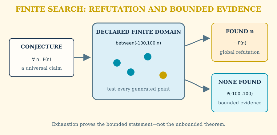
Examples suggest; proofs compel
The first values of a sequence can suggest a recurrence. Exhaustive search up to a bound can destroy a false conjecture. Neither establishes a universal theorem over an unbounded domain.
This boundary can be written directly:
:- use_module(library(between), [between/3]).
:- use_module(library(lists)).

counterexample_to_odd_square(N) :-
  between(1, 100, N),
  (1 is N mod 2),
  (Square is N * N),
  (Remainder is Square mod 2),
  (Remainder \= 1).
eyeprolog --goal 'counterexample_to_odd_square(N)' program.pl
No answer means only that no counterexample was found in the generated range
under the implemented arithmetic. The theorem that every odd integer has an
odd square needs an algebraic argument valid for an arbitrary integer:
(2k+1)^2 = 2(2k^2+2k)+1.
By contrast, if the claim concerns exactly the integers from 1 through 10,000, the finite exhaustive search can be a proof—provided the generator is complete, the predicate expresses the property correctly, and the arithmetic implementation is trusted.
One counterexample has asymmetric power
A universal statement falls to one valid counterexample. This makes finite search especially valuable for criticism. Testing associativity over random inputs offers evidence; finding one triple where associativity fails settles the negative question.
noncommuting_pair(A, B) :-
  matrix(A),
  matrix(B),
  matrix_multiply(A, B, AB),
  matrix_multiply(B, A, BA),
  (AB \= BA).
The example need not explain every failure of commutativity. Its existence is enough to refute the universal claim. This asymmetry between confirmation and refutation is one reason constraint solving, model finding, and property-based testing are so productive.
Finite model exploration
A finite structure consists of a finite carrier and interpretations of its operations and relations. EyeProlog can enumerate candidates, apply axioms as filters, and return models or countermodels. The method is mathematically serious because the scope is explicit.
For a carrier of three named elements, a binary operation table has nine entries. Searching all possible tables is finite but large. Algebraic laws can prune partial or complete candidates:
- closure restricts every output to the carrier;
- an identity fixes an entire row and column;
- commutativity identifies mirrored entries;
- associativity checks triples;
- inverse requirements constrain remaining cells.
The order of these constraints is operational mathematics. A strong law applied early may collapse the search space; the same law applied after full generation merely rejects enormous numbers of candidates.
Combinatorics is the anatomy of search
Search complexity is often a counting problem before it is a programming
problem. If a choice has n alternatives at each of k positions, naive
generation contains n^k leaves. If order does not matter, permutations may
be redundant. If partial choices already violate a constraint, pruning saves
an entire subtree.
This is why combinatorial examples are not toys. clpz-n-queens.pl exposes
the classic N-queens search through finite-domain constraints – genuinely
searched at four queens; its eight-queens goal instead checks a known witness
against the same model, without searching for it. Together with send-more-money.pl,
integer-partitions.pl, stirling-bell-numbers.pl,
and weighted-interval-scheduling.pl, they show different geometries of
choice: permutations, digit assignments, recursive decompositions, set
partitions, and ordered optimization.
For each search program, ask a mathematical question before a performance question:
What objects are being counted, and when do two execution branches denote the same mathematical object?
Only after answering that should one add indexing, reorder goals, or introduce an accumulator. Otherwise the program may optimize accidental multiplicity.
Numerical models and epistemic humility
The scientific examples combine logical rules with floating-point
calculations. beam-deflection.pl, orbital-transfer-design.pl,
competitive-enzyme-kinetics.pl, and least-squares-regression.pl encode
mathematical models of physical or statistical relationships.
A correct derivation inside such a model establishes a conditional:
given these measurements, equations, units, approximations, and thresholds, this conclusion follows under the implementation’s numeric semantics.
It does not establish that the sensor was calibrated, the model applies in this regime, omitted variables are negligible, or a floating-point result is an exact real number. The proof boundary should name these conditions rather than conceal them.
Exercises.
- Turn a familiar universal conjecture into a bounded counterexample search. State what a failure to find an answer does and does not prove.
- Estimate the naive search space of
send-more-money.pl, then identify each constraint that removes branches. - Use
examples/stirling-bell-numbers.plto connect a recurrence with the combinatorial objects it counts. - Design a finite carrier and search for a noncommutative operation with an identity.
- Choose one scientific example and list every premise outside pure logic: measurements, units, empirical law, approximation, and numeric behavior.
Checkpoint. Label a computation as one of: witness construction, counterexample, exhaustive finite-model check, bounded evidence, or numerical model evaluation. Write one sentence stating exactly what its success proves and what its failure leaves open.
30. What mathematics promises
Mathematics earns unusual trust because it makes its conditions inspectable. Once definitions, axioms, and inference rules are fixed, a valid proof does not negotiate with status, rhetoric, fashion, or desire. The conclusion either follows by the accepted rules or it does not.
That is perhaps the precise sense in which mathematics does not cheat us. It does not promise that our premises describe the world. It promises that we can ask whether the conclusion follows from them.
Conditional certainty
Every theorem is conditional, even when the conditions have become culturally invisible:
axioms + definitions + inference rules
  -> theorem
Every trustworthy EyeProlog conclusion has the same broad shape:
source facts + clauses + built-in semantics + execution assumptions
  -> ground answer + proof
The arrows are where rigor lives. A proof disciplines the transition from premises to conclusion. It cannot authenticate the premises merely by using them.
This yields four layers of trust:
- Source trust: are facts authentic, current, complete enough, and represented with the correct units and identity?
- Model trust: do the predicates and rules express the intended domain?
- Engine trust: do parsing, unification, built-ins, tabling, and proof generation implement the stated standards profile?
- Derivation trust: does this answer have a valid proof from this exact theory?
Explicit integrity relations expose contradictions and invalid states inside the supplied theory. Conformance tests address the implementation. Proof output addresses the derivation. Provenance, signatures, calibration, peer review, and domain validation address other layers. No single mechanism replaces the rest.
The dignity of a counterexample
Mathematics corrects itself through definitions and counterexamples. A false conjecture is not rescued by the beauty of its statement. One legitimate counterexample has standing against a thousand confirming cases.
Logic programming should preserve this culture. Write negative tests before the theory becomes emotionally expensive. Search boundary cases. Ask for forbidden states. Turn domain invariants into queryable integrity relations. Keep the failed model that forced a redesign.
A knowledge system becomes trustworthy not when it never changes, but when it can say:
- what it assumed;
- what followed;
- which evidence was used;
- which counterexample broke the former rule;
- when the theory changed; and
- which past conclusions belonged to which version.
This is mathematical honesty translated into engineering practice.
The limits are part of the truth
Gödel, Church, and Turing did not diminish mathematics by proving limits. They made informal hopes precise enough to refute. There is no complete effective method that settles every sufficiently expressive mathematical question. No amount of faster hardware turns an undecidable general problem into a decidable one.
EyeProlog has smaller, immediate limits:
- some relations have infinitely many answers;
- depth-first search may pursue an unproductive branch;
- mode-sensitive built-ins are not omnidirectional equations;
- negation as failure is not classical negation;
- floating-point arithmetic is not exact real arithmetic;
- tabling terminates only when the relevant call and answer spaces stabilize;
- proof output explains successful derivations, not every failed search path;
- the language cannot prove arbitrary metatheorems about its own programs.
Naming these limits is not an apology. A trustworthy formal tool states the edge of its guarantee.
Mathematics as a style of care
The deepest lesson is methodological. Mathematics asks us to separate:
- a name from its definition;
- an example from a proof;
- existence from construction;
- a theorem from its converse;
- syntax from semantics;
- equality from resemblance;
- local evidence from a universal claim;
- correctness from termination;
- the model from the world.
Those separations are exactly what good logic programming requires. A predicate must have a sentence. A recursive clause must have an invariant and a termination argument. A finite search must declare its domain. An aggregate must have a bounded subsearch. A decision must retain its premises. A proof must remain attached to the theory version that licensed it.
The result is not certainty about everything. It is something more useful: certainty whose boundary is visible.
A final program-reading ritual
Before trusting an EyeProlog conclusion, ask:
- What does the ground answer say in the domain?
- Which facts and rules support it?
- Which facts came from outside the theory?
- Which built-ins contribute extra semantics?
- Was the search domain finite, and why?
- Could goal or clause order hide an answer?
- Does negation mean absence of proof or an explicit opposite?
- What invariant justifies each recursive relation?
- What counterexample would overturn the model?
- Can the result be reconstructed under the same source and theory version?
That ritual captures the discipline. State a small theory. Ask a precise question. Let the machine search. Inspect the witness. Challenge the premises. Preserve the proof.
Exercises.
- Take one policy example and classify every dependency under the four layers of trust.
- Write a conclusion that is logically valid from false premises. Explain why proof checking alone cannot repair it.
- Add version and provenance facts to a scientific example and make them visible in its explanation.
- Find one claim in your own program for which tests provide evidence but not proof. State the missing universal argument.
- Write a one-page “trust contract” for an embedded EyeProlog service: accepted sources, model scope, numeric assumptions, resource bounds, proof retention, and known limits.
Checkpoint. Take one strong conclusion and prefix it with every condition on which it depends: source authenticity, model scope, built-in semantics, finite search, theory version, and derivation validity. If the qualified claim still matters, the model has earned its confidence honestly.
Part VI summary
Part VI placed logic programming inside the longer history of mathematics:
- a ground answer can carry the witness of an existential claim;
- definite-program closure connects proof search with least-model semantics;
- recursive definitions and inductive proofs often share a constructor skeleton;
- correctness, completeness, and termination are independent obligations;
- unification solves equations in a free term algebra, not every domain;
- symmetry and canonical form remove representational duplicates;
- finite search is experimental mathematics whose scope must be stated;
- formal certainty is conditional on sources, models, engines, and rules.
You should now be able to distinguish computation from proof, bounded evidence from a universal theorem, syntactic equality from mathematical equivalence, and valid derivation from trustworthy premises.
Historical note: mathematics examines its own methods
This arc begins before electronic computing. Hilbert’s program made formal proof and consistency mathematical objects. Gödel established limits for sufficiently expressive effective axiomatic systems. Church and Turing made effective calculability precise enough to prove that some general decision problems have no algorithm. Herbrand and Robinson supplied ideas that became central to automated first-order deduction.
Logic programming belongs to this history because it operationalizes a restricted proof discipline. It does not erase the limit results or turn every existence proof into an efficient witness generator. It gives a small region where propositions, substitutions, proof steps, and computations can be inspected together.
The deeper inheritance is a style of honesty. Mathematics advanced by proving not only more statements but also where methods fail, separating truth, provability, decidability, and computation. EyeProlog’s finite bounds, mode restrictions, search risks, and trust boundaries belong inside its account for the same reason: limits are part of the result, not fine print.
Part VII — The reasoning laboratory
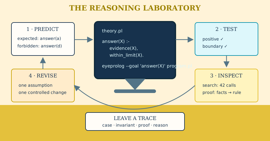
The final craft is experimental without being careless. A logic programmer works like a mathematician at a blackboard and an engineer at a test bench: state a claim precisely, derive consequences, seek counterexamples, measure the computation, and preserve enough evidence for another person to repeat the work.
The reasoning laboratory turns these ideas into a daily discipline. It adds no new language feature; it shows how to make theories survive change.
31. Testing a theory
A conventional unit test often presents an input to a function and compares one returned value with an expected value. A relational program needs a wider test vocabulary. One call may have several answers, no answer, duplicate proofs, or different useful modes. Correctness includes the answer set, the absence of forbidden answers, the shape of witnesses, and the finiteness of the intended search.
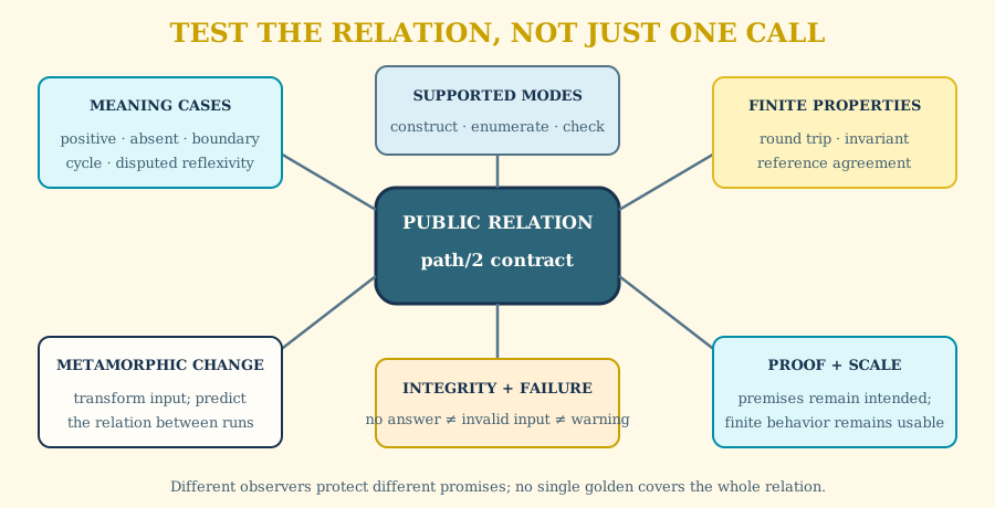
Begin with a semantic test table
Before writing test code, make a table in domain language:
| Case | Given | Question | Expected | Why this case matters |
|---|---|---|---|---|
| direct | edge(a,b) |
path from a to b? |
yes | base clause |
| composed | a→b→c |
path from a to c? |
yes | recursive clause |
| absent | disconnected d |
path from a to d? |
no | false positive |
| cycle | c→a |
all destinations from a? |
finite set | tabling or visited state |
| reflexive | no explicit loop | path from a to a? |
design choice | relation boundary |
The last row is especially valuable. Many bugs are not implementation mistakes but unresolved meanings. Does a path require at least one edge, or may it be empty? No test framework can choose the definition for you.
Positive and negative observers
Queries naturally record positive expectations:
:- use_module(library(lists)).

edge(a, b).
edge(b, c).

path(X, Y) :- edge(X, Y).
path(X, Z) :- edge(X, Y), path(Y, Z).
eyeprolog --goal 'path(a, b)' program.pl
eyeprolog --goal 'path(a, c)' program.pl
To make an expected absence visible, define a finite observer:
unexpected_path :-
  path(a, d).

expected_absence :-
  \+ unexpected_path.
eyeprolog --goal 'expected_absence' program.pl
This is a test over a ground, terminating goal. It does not turn negation as failure into classical negation; it records that this finite theory derives no such path.
For a reusable package, prefer a dedicated test program that loads or reproduces the relevant theory and declares only test queries. For a small example, the golden answer file is an executable specification of the expected answer set.
Test the relation from more than one mode
Suppose append/3 is intended both to concatenate and to split:
eyeprolog --goal 'append([a, b], [c], Whole)' program.pl
eyeprolog --goal 'append(Prefix, Suffix, [a, b])' program.pl
The first call should construct one list. The second should enumerate three splits. Testing only the first mode would miss a regression in relational generality; testing the completely open mode would request an infinite relation and prove little beyond the absence of a useful bound.
For every public predicate, record:
- the principal mode;
- any secondary supported modes;
- modes that are meaningful but intentionally unsupported;
- calls expected to be finite;
- calls whose answer order is part of the observable contract.
Keep this design close to the clauses in comments or tests, and exercise each supported call pattern directly.
Properties over finite domains
Examples test selected points. A finite generated property tests every point in a declared scope:
:- use_module(library(between), [between/3]).
:- use_module(library(lists)).

double(N, D) :- (D is N + N).

double_is_even(N) :-
  double(N, D),
  (0 is D mod 2).

bounded_double_law :-
  \+ bounded_double_counterexample.

bounded_double_counterexample :-
  between(-100, 100, N),
  \+ double_is_even(N).
eyeprolog --goal 'bounded_double_law' program.pl
This is exhaustive for the 201 generated integers, not for all integers.
Naming the predicate bounded_double_law/0 keeps the scope honest.
Useful finite properties include:
- round trips: parse then render, or encode then decode;
- preservation: normalization keeps the represented value;
- idempotence: normalizing twice equals normalizing once;
- symmetry: an undirected adjacency relation works in both directions;
- invariants: every generated plan state is safe;
- agreement: a simple reference relation and an optimized relation return the same bounded answer set.
Metamorphic tests
Sometimes the correct answer is hard to list, but a controlled change has a predictable effect. These are metamorphic tests.
If an isolated graph vertex is added, existing reachability answers should not change. If every edge cost is multiplied by a positive constant, the cheapest route should retain the same vertices. If the order of source facts changes, the set of logical answers should remain unchanged even if their discovery order changes.
A metamorphic test states a relation between runs. It is particularly useful for optimizations because it checks a preserved invariant rather than one frozen implementation trace.
Proof regression and answer regression
An answer golden asks, “Did the public conclusions change?” A proof golden asks, “Did their supporting derivations change?”
Proof changes may be desirable after introducing a clearer helper. They may also reveal that a decision now depends on an unintended fact. Treat proof goldens as reviewed evidence, not snapshots updated automatically whenever a test fails.
Use answer regression broadly. Use proof regression selectively where provenance, explanation, or policy accountability is part of the product.
Test failures, integrity results, and warnings
Three outcomes carry different meanings:
- an ordinary query has no answer: the relation did not establish that goal;
- an integrity query succeeds: the supplied input violates a forbidden condition;
--warningsreports unstratified negation: execution may proceed, but the program crosses a portability and semantic boundary.
A mature suite covers all three. Include malformed source in parser tests, inconsistent source in integrity-query tests, and semantically dubious dependency cycles in warning tests.
A release-quality test matrix
Before releasing a theory or embedded service, cover:
| Dimension | Minimum evidence |
|---|---|
| Meaning | one positive, one absent, and one boundary case per public relation |
| Modes | every documented mode; explicit rejection or warning for unsafe uses |
| Recursion | base case, multi-step case, cycle, and termination argument |
| Search | smallest witness, competing witnesses, ties, and empty domain |
| Negation | ground success, ground failure, and stratification check |
| Aggregation | empty, singleton, duplicates, and deterministic tie handling |
| Integrity | each invalid state is detected and valid input is not misclassified |
| Proof | representative derivation with source premises visible |
| Scale | a case large enough to expose indexing or table behavior |
| Reproducibility | fixed time, source version, stable fixtures, and clean output |
Exercises.
- Build the semantic test table for
ancestor/2, including a cycle and a disputed reflexive case. - Write bounded commutativity and associativity tests for a finite operation table. Explain why one is cheaper.
- Create a metamorphic test for a route planner.
- Choose one proof golden and identify changes that should be accepted versus changes that should block a release.
- Design a test that distinguishes “no answer” from “invalid input theory.”
Checkpoint. Assemble a minimum release matrix for one public relation: positive, absent, boundary, alternate mode, recursive or cyclic, integrity, proof, and scale cases. State which expected outputs should be exact goldens.
32. Debugging by meaning, search, and proof
Debugging a logic program is difficult when every symptom is described as “the query failed.” Failure can mean the fact is absent, a variable was bound too early, a built-in ran outside its mode, a negative goal saw an unintended answer, recursion did not reach its base case, or the original relation was misstated.
Use four views in a fixed order:
- meaning: what should a ground instance say?
- bindings: what is known before each goal?
- search: which alternatives are explored, repeated, or pruned?
- proof: which successful premises support the observed answer?
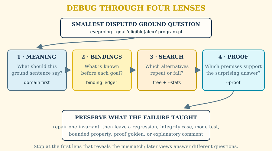
Reduce to the smallest disputed ground question
Do not begin with an open query that prints hundreds of answers. Name one conclusion that is missing or surprising:
eyeprolog --goal 'eligible(alex)' program.pl
Then expand only the clause intended to prove it. Replace broad generators with the relevant ground facts. A small ground question removes accidental branching and makes every failed subgoal discussable.
If the ground question is itself ambiguous, stop debugging the implementation. Rewrite the domain sentence first.
Follow bindings from left to right
Consider:
:- use_module(library(lists)).

eligible(Person) :-
  (Age >= 18),
  age(Person, Age).
The intended mathematics is easy to recognize, but >=/2 sees an unbound
Age. Write a binding ledger:
| Before goal | Goal | Bindings produced |
|---|---|---|
| none | Age >= 18 |
none; not ready |
| — | age(Person,Age) |
never productively reached |
Reordering the goals repairs the operational mode:
:- use_module(library(lists)).

eligible(Person) :-
  age(Person, Age),
  (Age >= 18).
For a clause with five goals, the ledger is often more revealing than staring at the source. Record structures as well as scalar bindings: a variable may be bound to an improper list or a compound term whose inner variables remain open.
Use a symptom atlas
No answers
- Confirm the queried predicate name and arity.
- Ground one expected answer and locate a clause whose head unifies with it.
- Walk the body with a binding ledger.
- Check readiness of arithmetic, string, list, and term built-ins.
- Inspect whether a negative goal is too early.
- Verify that a base clause is reachable.
Too many answers
- State which answer violates the domain sentence.
- Find its proof and identify the first overbroad premise.
- Look for missing joins: the same conceptual entity may use two variables where one shared variable was intended.
- Check whether a closed-world assumption was omitted.
- Decide whether duplicate answers or duplicate proofs are the real issue.
Right answers, wrong order
- Inspect clause order and generator order.
- Identify
once/1or aggregate tie-breaking that makes order observable. - Do not confuse order-sensitive behavior with declarative completeness.
Nontermination or explosive search
- Name the intended finite domain.
- Identify the recursive call and its decreasing measure, or the finite tabled call/answer space.
- Move selective generators and ready filters earlier.
- Check for terms that grow on every recursive call.
- Run with
--statsand compare one controlled revision at a time.
A surprising proof
- Verify that the answer itself is intended.
- Find the earliest source premise that should not have participated.
- Distinguish a misleading helper name from a semantically wrong clause.
- Check whether two source versions or contexts were accidentally combined.
Create diagnostic relations
Temporary helpers can expose intermediate concepts:
:- use_module(library(lists)).

candidate_debug(Person, Age) :-
  age(Person, Age).

adult_debug(Person, Age) :-
  candidate_debug(Person, Age),
  (Age >= 18).
eyeprolog --goal 'candidate_debug(Person, Age)' program.pl
eyeprolog --goal 'adult_debug(Person, Age)' program.pl
Once the fault is understood, either remove the helper or rename it as a
permanent domain concept. Do not leave debug2/3 archaeology in a theory whose
proofs people must read.
Compare specification and implementation
For a bounded domain, write a deliberately simple reference relation and compare it with the optimized one. The reference may be slow; its purpose is clarity.
:- use_module(library(between), [between/3]).
:- use_module(library(lists)).

reference_square(N, S) :-
  between(0, 20, N),
  (S is N * N).

optimized_square(N, S) :-
  between(0, 20, N),
  (S is N * N).

disagreement(N, S) :-
  reference_square(N, S),
  \+ optimized_square(N, S).
eyeprolog --goal 'disagreement(N, S)' program.pl
A complete equivalence check needs both directions and must account for duplicates if proof multiplicity matters. Within a finite domain, differential testing is a powerful guard during program transformation.
Read statistics as questions
--stats reports work, not meaning. A high solution count may be necessary or
may indicate a generator that should be constrained. Many table hits may show
effective reuse; many distinct table entries may reveal an argument that
prevents calls from sharing table entries. On the Node CLI it also reports current heap use,
non-young/old-generation use, the amount currently compared with the memory
guard, resident-set size, and the soft and hard memory ceilings in bytes. These
memory figures are printed even when execution ends by raising a Prolog error.
--stats is an end-of-run summary. For a deliberately non-terminating or very
long computation, call the EyeProlog extension statistics/0 at the points
where a live snapshot is useful. For example, a long-running loop can include
statistics as one of its goals, as in loop :- work, statistics, loop.
statistics/0 writes the current solver counters and memory figures
immediately to the current output stream. statistics/2 makes an individual
value available to the program, for example
statistics(memory_guard_used_bytes, Used). With an unbound first argument it
enumerates the available statistic keys and values. An atom that is not an
available key raises domain_error(statistics_key, Key) rather than silently
failing. These predicates are EyeProlog observability extensions and are not
available under --iso-strict.
Compare statistics only between runs with the same query, data, and observable answer contract. A faster program that silently loses answers is not an optimization.
Preserve the failure that taught you
Every repaired defect should leave behind one of:
- a new positive or negative case;
- an integrity regression;
- a documented mode and tests for that call pattern;
- a bounded property;
- a proof golden;
- a comment stating a non-obvious invariant.
Otherwise the repository remembers the repair but forgets the reason.
Exercises.
- Deliberately misorder a numeric filter and diagnose it with a binding ledger.
- Introduce a missing-variable join into a two-relation rule. Use the proof of one false positive to locate it.
- Create a recursive term-growing rule, then state why tabling cannot make its answer space finite.
- Compare statistics before and after moving an invariant calculation out of recursion.
- Write a bidirectional bounded equivalence check for two list relations.
Checkpoint. Preserve one defect as a regression. Record the smallest disputed ground question, expected answer, first incorrect binding or search choice, repaired invariant, and test that would fail if the defect returned.
33. A pattern catalog for reasoning
A pattern is not a copied code fragment. It is a recurring arrangement of meaning, representation, and control that solves a named design problem. The following patterns collect constructions that are especially useful in practice.
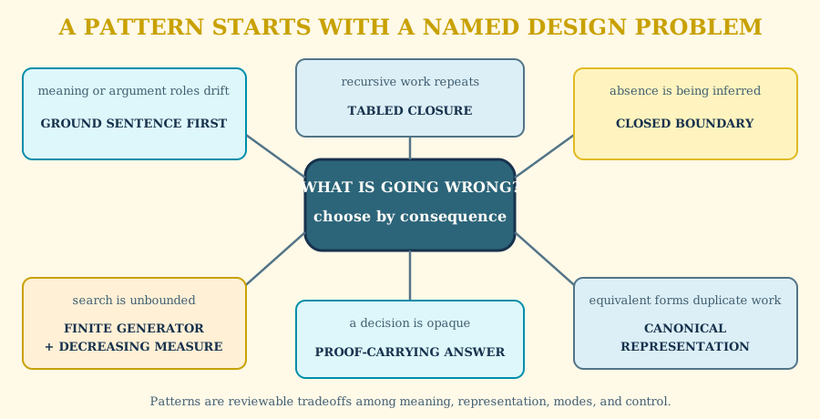
Pattern 1: Ground sentence first
Problem: a predicate’s argument order and meaning drift while rules are being written.
Form: write one representative ground fact and read it aloud before adding variables.
:- use_module(library(lists)).

assigned_badge(alex, badge_17).
Consequence: argument roles become reviewable; modes and indexes can be discussed against a stable sentence.
Pattern 2: Normalize at the boundary
Problem: spelling, aliases, units, or source-specific terms leak into every domain rule.
Form: retain source facts, derive one canonical vocabulary, and make core rules depend only on the normalized layer.
:- use_module(library(strings)).
:- use_module(library(lists)).

source_role(person_7, 'Doctor').

canonical_role(Person, clinician) :-
  source_role(Person, Text),
  lowercase(Text, doctor).
Consequence: adapters change independently from policy; proofs still trace back to source data.
Pattern 3: Generate, constrain, describe
Problem: a search relation mixes candidate production, pruning, and explanation until none can be reasoned about separately.
Form: generate a finite candidate, apply the cheapest selective constraints in dependency order, then construct a witness or reason.
:- use_module(library(between), [between/3]).
:- use_module(library(lists)).

chosen_pair(pair(X, Y), reason(sum_is_ten)) :-
  between(0, 10, X),
  between(X, 10, Y),
  (10 is X + Y).
Consequence: the search domain and each pruning step are visible.
Pattern 4: Carry the witness
Problem: a Boolean-like conclusion proves existence but loses the object needed for explanation or later computation.
Form: add a structured output containing the path, assignment, schedule, or evidence summary.
:- use_module(library(lists)).

path(X, Y, [X, Y]) :- edge(X, Y).
path(X, Z, [X | Rest]) :-
  edge(X, Y),
  path(Y, Z, Rest).
Consequence: answers become constructive; witness size and duplicate paths become explicit design concerns.
Pattern 5: Bound absence
Problem: the domain needs a negative conclusion, but absence is meaningful only after a complete finite search.
Form: bind the subject and finite scope before \+/1; isolate the
closed-world step behind a clearly named predicate.
unregistered(Person) :-
  person(Person),
  \+ registered(Person).
Consequence: the closed-world assumption has one reviewable home. It must not be mistaken for an explicit fact that the person is not registered.
Pattern 6: Explicit state transition
Problem: planning or interpretation appears to require mutable state.
Form: represent the old and new states as terms related by an action.
step(state(Room, outside), enter(Room), state(Room, inside)).
Consequence: histories are ordinary lists, transitions can be queried, and the state representation exposes invariants.
Pattern 7: Fixed-point closure
Problem: reachability, inheritance, or dataflow revisits the same finite subquestions.
Form: state the positive recursive relation directly and let eligible components be tabled.
depends(X, Y) :- direct_dependency(X, Y).
depends(X, Z) :- direct_dependency(X, Y), depends(Y, Z).
Consequence: termination rests on a finite call and answer space, not on pretending the graph is acyclic.
Pattern 8: Proof façade
Problem: low-level helper clauses produce technically correct but unreadable explanations.
Form: introduce stable domain concepts and a small public decision relation whose premises are meaningful reasons.
within_limit(Device) :-
  reading(Device, Value),
  maximum(Max),
  (Value =< Max).

status(Device, safe) :-
  within_limit(Device).
Consequence: internal calculations remain available, while the successful proof reads in domain vocabulary.
Pattern 9: Integrity before inference
Problem: contradictory or impossible input would make ordinary conclusions misleading.
Form: encode forbidden combinations as ordinary relations with diagnostic arguments.
:- use_module(library(lists)).

invalid_badge_assignment(Badge, PersonA, PersonB) :-
  assigned_badge(PersonA, Badge),
  assigned_badge(PersonB, Badge),
  (PersonA \= PersonB).
Consequence: callers can collect every defect, and a host that requires validated input can query this relation before it requests trusted decisions. The rejection policy remains explicit rather than being hidden in clause-head syntax.
Pattern 10: Version the evidence boundary
Problem: an answer can be reproduced only if its facts, rules, and external semantics are known.
Form: retain source snapshot, theory version, adapter version, and relevant clock or numeric assumptions beside the proof.
theory_version("2026-07-24").
source_snapshot("telemetry-0042").
numeric_model(ieee_754_double).
Consequence: an old decision can be reconstructed under the system that actually made it rather than silently rerun under today’s theory.
Anti-patterns
The unbounded open generator. A relation is queried with every argument free even though its mathematical extension is infinite.
The premature test. A mode-sensitive built-in or negative goal appears before the goals that bind its inputs.
The accidental Cartesian product. Two goals use different variables for what should be the same entity.
The opaque mega-clause. One rule performs normalization, search, policy, and explanation with no named intermediate concepts.
The Boolean witness eraser. A relation returns only yes after doing the
work needed to construct a useful path or reason.
The silent closed world. Failure to derive a fact is used as its opposite without documenting finite scope and completeness assumptions.
The proof-hostile helper. Names such as step3/2 or tmp/4 expose an
implementation sequence instead of a domain idea.
The optimization by answer loss. once/1, early aggregation, or reordered
search makes a benchmark faster by changing the public answer contract.
The floating theorem. A numerical result is described as mathematically exact without naming units, approximation, or host floating-point behavior.
The timeless decision. Sources and rules change, but conclusions retain no snapshot or theory version.
Selecting patterns
Patterns compose. A robust decision service often uses:
normalize at the boundary
  -> generate, constrain, describe
  -> carry the witness
  -> proof façade
  -> integrity before inference
  -> version the evidence boundary
Do not apply every pattern mechanically. A three-fact teaching example does not need six architectural layers. Introduce a pattern when its named problem is present, and keep the smallest theory that makes meaning and control clear.
Exercises.
- Find three patterns and two anti-patterns in an existing large example.
- Refactor an opaque rule into boundary, concept, and decision layers; compare proofs before and after.
- Add witness carrying to a Boolean reachability relation and analyze the new duplicate-answer behavior.
- Replace a silent closed-world decision with a named bounded-absence helper.
- Write a versioned evidence envelope for the Chapter 25 decision service.
Checkpoint. Select the smallest set of patterns that solves a real problem in one theory. For every selected pattern, name the pressure that justifies it; remove any layer that exists only because the catalog made it available.
Part VII summary
Part VII made theory development repeatable:
- semantic test tables settle meanings before test mechanics;
- positive, absent, boundary, cycle, and scale cases cover different risks;
- bounded properties and metamorphic relations test more than selected points;
- answer and proof goldens protect different contracts;
- binding ledgers diagnose readiness and accidental joins;
- debugging moves from meaning to bindings, search, and proof;
- named patterns connect recurring problems to reusable relational forms;
- every repaired defect should leave a case, invariant, integrity check, or explanation.
You should now be able to design a release-quality test matrix, reduce a surprising result to one ground question, compare a reference relation with an optimized relation, and recognize productive patterns and anti-patterns.
Historical note: executable specifications learn to remember
Logic programs have long stood between specification and implementation. That made testing both easier and subtler: a ground clause could serve as an example, yet a relation might have several modes and an answer set rather than one returned value. Testing practice absorbed ideas from theorem proving, database validation, software regression, and property-oriented testing.
The repository form of this practice is historically significant in its quiet way. A theory, exact answer file, proof file, conformance corpus, and version tag preserve not only a program but expectations about its meaning. Regression tests make old decisions reviewable; property tests seek counterexamples; metamorphic tests state what remains invariant across controlled change.
Patterns complete the cycle by naming recurring design knowledge. Sterling and Shapiro’s craft-oriented presentation helped establish that expertise lives in constructions and transformations, not syntax alone. The reasoning laboratory extends that attitude into maintenance: prediction, execution, evidence, and revision form one method, and the failure that taught a lesson becomes executable memory.
Part VIII — Standard Prolog in practice
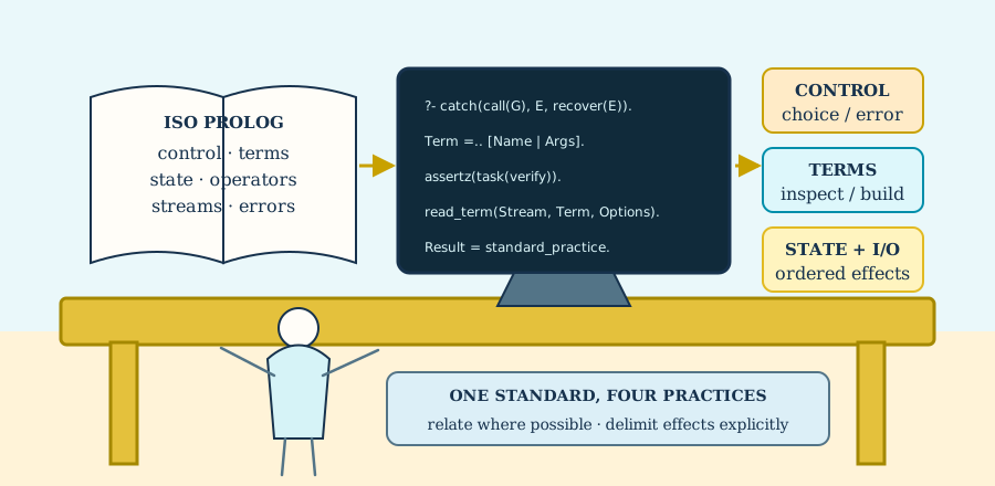
The supported ISO Prolog profile includes processor-facing facilities that
become important in reusable libraries, language tools, long-running
applications, and file boundaries. Earlier chapters use its relational core;
this part makes control, reflection, state, operators, and streams explicit.
For Part 1 portability work, EyeProlog also provides a strict core mode:
--iso-strict on the CLI or isoStrict: true in the JavaScript API restricts
the language/runtime surface to ISO/IEC 13211-1:1995 plus Technical Corrigenda
1–3. The processor character set is an implementation-defined choice shared by
normal and strict profiles: EyeProlog uses Unicode scalar values U+0000..U+10FFFF
excluding surrogates, with the scalar value as the collating-sequence integer.
Strict mode restricts implementation-specific language facilities, but it does
not narrow this processor-defined character repertoire. Isolation and error cases live in test/conformance/cases/iso/.
The examples here compose those operations into programs worth changing and
rerunning.
These facilities do not all have the same declarative character. Term inspection and atomic conversion are relations. Cut commits to an operational choice. Dynamic updates and stream operations change solver-owned state. Use the pure relation when it expresses the problem; introduce control or effects at a named boundary.
34. Control, exceptions, and grouped solutions
The control predicates accept goals as arguments. call/1 invokes a callable
term, and call/2-8 appends arguments to a callable closure. The expanded goal
runs in the current search continuation, so a direct goal and its meta-called
form expose the same remaining alternatives; the meta-call still establishes
its own cut boundary. once/1 keeps its first solution, and !/0 commits
within the clause that contains it. If-then-else commits to the first successful
condition:
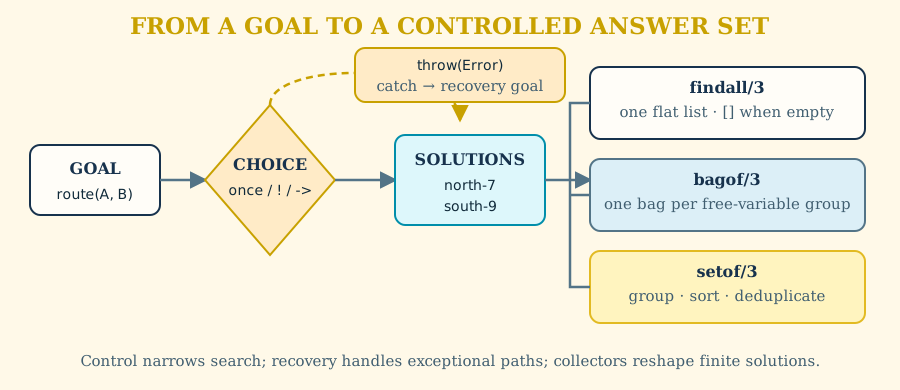
travel_status(From, To, Status) :-
  (route(From, To) -> Status = connected ; Status = disconnected).
once(Goal) is a local request for one solution. Cut is lower level: it
discards alternatives created since entry into the current predicate call.
The two can produce the same first answer without expressing the same control
boundary. Keep cut close to the choice it documents and test the complete
answer set before and after introducing it. A cut executed inside a predicate
called by one disjunction branch remains local to that predicate: if the branch
later fails, Left ; Right must still try Right. This also holds when a
cut-bearing validation helper is called from a branch driven by a generator
such as between/3: the helper’s own cut still stays local to it.
Exceptions separate an exceptional call from ordinary logical failure:
require_route(From, To) :-
  (route(From, To) -> true ; throw(no_route(From, To))).

checked_route(From, To, Result) :-
  catch(
    (require_route(From, To), Result = accepted),
    no_route(From, To),
    Result = rejected
  ).
The catcher is unified with the thrown term. A matching recovery goal runs in
the environment at the catch/3 boundary; unrelated exceptions continue
outward. Prefer failure for an expected negative answer, such as a route that
does not exist. Throw when a caller cannot safely interpret the computation,
for example malformed input or an unavailable required resource. ISO
instantiation, type, domain, permission, representation, and evaluation errors
follow this same exception path.
Normal EyeProlog also provides call_cleanup(Goal, Cleanup) and
setup_call_cleanup(Setup, Goal, Cleanup). Cleanup is run exactly once when the
protected search completes deterministically, is exhausted, is cut or otherwise
pruned, top-level answer enumeration is abandoned, or an exception unwinds the
search. setup_call_cleanup/3 runs Setup once and installs Cleanup only after
Setup succeeds. On cut or ordinary pruning Cleanup sees the current Goal
bindings; on exception unwind the Goal bindings have been removed and Cleanup
sees the Setup environment. When a deterministic protected goal runs Cleanup
before yielding, substitutions produced by a successful Cleanup are included in
that answer. Cleanup failure is ignored, and an exception already being
propagated takes precedence over a cleanup exception. Nested cleanups run
inside-out. These two controls are EyeProlog extensions and are absent from
--iso-strict.
Collection also makes search boundaries explicit. findall/3 returns one list
and existentially closes variables that occur only in its goal. bagof/3
instead creates a group for each binding of a free variable and fails when
there are no solutions. setof/3 has the same grouping rule, then sorts and
deduplicates each group. The ^/2 notation marks a goal variable existential:
:- use_module(library(lists)).

regional_total(Region, Total) :-
  bagof(Amount, Seller^sale(Region, Seller, Amount), Amounts),
  sum_amounts(Amounts, Total).
Here Region deliberately remains free and produces one answer per region;
Seller is hidden from grouping. This distinction matters whenever a
collection unexpectedly arrives as several answers.
Integer arithmetic has similarly precise choices. // truncates the quotient
toward zero, while Corrigendum 2’s div takes the mathematical floor. With a
positive divisor, mod returns a nonnegative modulo while rem keeps the
dividend’s sign. For -7 and 3, // is -2, div is -3, and the two
remainders are 2 and -1. Bitwise conjunction, disjunction, exclusive-or,
complement, and shifts require integers.
Run the focused examples:
iso-control-and-errors.plcoverscall/1,once/1, cut, if-then-else, and recovery;iso-grouped-solutions.plcontrasts the three collectors and inspects a source clause; andiso-integer-arithmetic.plmakes division and bit-operation results visible.
Checkpoint. Explain why bagof(Amount, sale(Region, Seller, Amount), X)
groups on both Region and Seller, then write the existential qualification
that groups only on Region. Name one expected absence that should fail and
one broken precondition that should throw.
35. Reflective terms and atomic conversion
Ordinary pattern matching should remain the first choice when term shape is known. Reflective predicates are valuable when the shape itself is input: generic walkers, schema checkers, interpreters, and source transformations.
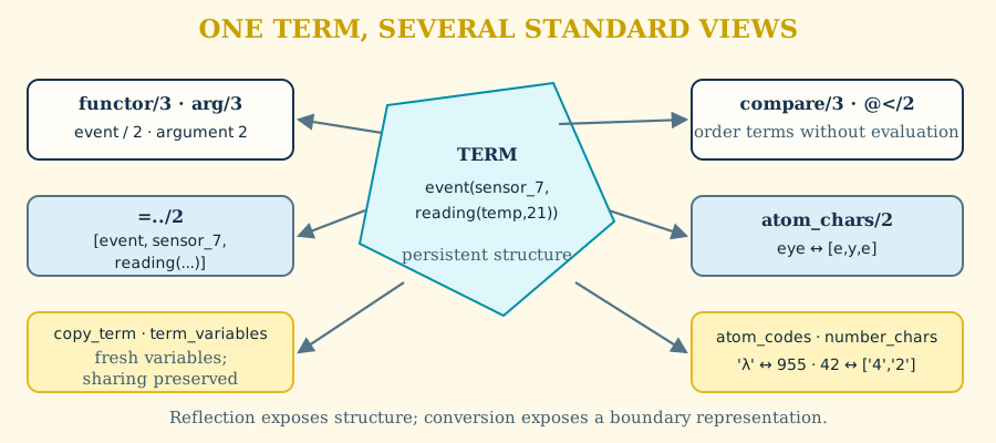
functor/3 relates a term to its name and arity. arg/3 selects a one-based
argument. =../2—traditionally called univ—relates a term to a list whose
head is the functor and whose tail contains the arguments:
term_shape(Term, shape(Name, Arity, Arguments)) :-
  functor(Term, Name, Arity),
  (Term =.. [Name | Arguments]).
In a construction mode, functor/3 creates a term with fresh arguments and
=../2 rebuilds a term from a proper list. Their ISO errors are useful
guardrails: an unknown functor name, negative arity, partial univ list, or
uninstantiated required argument is not silently treated as failure.
copy_term/2 preserves sharing inside a term while replacing its variables
with fresh ones. term_variables/2 returns each distinct variable in
first-occurrence order. Identity predicates make the distinction observable:
==/2 tests whether two resolved terms are identical without binding them;
\==/2 is its negation. =/2 still performs unification, while
unify_with_occurs_check/2 explicitly rejects cyclic bindings.
The standard term-order family—compare/3, @</2, @=</2, @>/2, and
@>=/2—compares terms without evaluating arithmetic. Do not replace
3 + 4 < 8 with 3 + 4 @< 8: the former evaluates numbers and the latter
orders syntax.
Atomic conversion predicates expose reversible representations:
atom_concat/3joins an atom or solves a sufficiently instantiated split;sub_atom/5relates a source to before, length, after, and fragment;atom_chars/2andatom_codes/2use character atoms or Unicode codes;char_code/2converts one character; andnumber_chars/2andnumber_codes/2parse or render ISO numbers.
These are atom relations, distinct from the EyeProlog library predicates whose
historical names contain string. Quoted atoms such as 'λ' remain atoms;
with the default flag, "λ" denotes the character list ['λ'].
iso-reflective-terms.pl
walks through shape, rebuilding, fresh copying, variables, and order.
iso-atomic-conversion.pl
demonstrates both conversion directions and every three-character sub-atom of
eyeprolog.
Checkpoint. Given pair(X, X), predict the variable list before and after
copy_term/2. Then explain why atom_codes/2 belongs at a text boundary
rather than throughout a domain theory.
36. Dynamic predicates, directives, and operators
A dynamic predicate is a mutable clause store owned by one solver run. Declare it before updates:
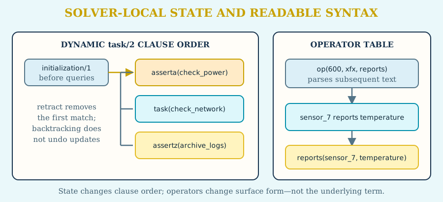
:- dynamic(task/2).

prepare_queue :-
  asserta(task(check_power, urgent)),
  assertz(task(check_network, normal)).
asserta/1 inserts at the beginning and assertz/1 at the end. retract/1
removes the first unifying clause and can be retried for later matches.
abolish/1 removes a dynamic procedure. clause/2 inspects accessible
clauses, while current_predicate/1 enumerates or tests predicate indicators.
Static and private built-in procedures are protected by permission errors.
Updates are ordered effects, not pure logical conclusions, and they are not
undone by ordinary backtracking: later goals observe a changed database. Each
update invalidates cached tabled and ground-chain answers, and rule changes
refresh recursion and negation analysis before later goals continue. Keep them
in a narrow lifecycle layer.
The queue example performs setup in initialization/1, so query order does not
determine its state:
:- initialization(prepare_queue).
Initialization runs after preparation and before host queries. include/1
expands a source file in place; ensure_loaded/1 loads the same designation at
most once. multifile/1 and discontiguous/1 document permitted clause
layout. Prolog flags and character conversions are also solver-scoped and
should be set deliberately near the boundary that relies on them.
Operators offer readable syntax without adding a new data model:
:- op(600, xfx, reports).

sensor_7 reports temperature.
The fact is exactly reports(sensor_7, temperature). Priority determines
binding strength, and fx, fy, xf, yf, xfx, xfy, and yfx
determine position and associativity. current_op/3 inspects the table;
op(0, Specifier, Name) removes a definition. Because declarations affect
parsing of subsequent text, place them before their first use. ISO argument
syntax also permits an atom that is currently an operator to appear directly
as a functional argument or list element, so forms such as
current_op(Priority, Specifier, :-) and [:-,-] are valid without quoting
or parenthesizing those operator atoms. A current operator atom may likewise
be the complete content of parentheses or curly brackets: (+) denotes the
atom +, and {*} denotes the curly term {}(*). Term output observes the
same context rules: with quoted(true), an operator atom is not quoted merely
because it occurs as a functional argument, list element, or sole curly-bracket
content. Thus writeq({*}) emits {*}, writeq([:-,-]) emits [:-,-], and
writeq(f(;,'|',';;')) emits f(;,'|',';;'); the bar stays quoted because
ISO treats the unquoted | token as a list separator rather than an atom.
The ISO initial operator table also
contains ?- at priority 1200 with specifier fx, so
current_op(1200, fx, ?-) succeeds. EyeProlog’s embedded quad syntax permits
an optional label before the query marker (Label ?- Query.); supporting that
syntax additionally exposes ?- at priority 1200 with specifier xfx as an
implementation-specific operator. Consequently
current_op(Priority, Specifier, ?-) enumerates both definitions. At top level in the normal EyeProlog profile, the quad marker is recognized
from the parsed ?-/1 or ?-/2 term rather than from one privileged surface
spelling. Thus Label ?- Query., ?-(Label, Query)., mixed forms such as
?-((Label), Query)., quoted-functor notation, and a parenthesized whole
(?-(Label, Query)). denote the same quad when followed by indented answer
descriptions. Label itself is parsed with the ordinary Prolog term grammar:
there is no quad-specific comma or metadata syntax. The runner requires the
resulting first argument to be ground; if it is not, that quad is reported as
BAD_ID and later quads are still processed. In --iso-strict mode this quad
interpretation is disabled, and ?-/2 remains ordinary Prolog term syntax.
Run iso-dynamic-database.pl
for an explicitly stateful queue and
iso-operators.pl
to see custom notation decomposed back into an ordinary term.
Checkpoint. State the final clause order after one asserta/1 and two
assertz/1 calls. Then rewrite one custom-operator fact in canonical
functor notation and verify it with =../2.
37. Streams and term I/O
Streams are handles to ordered input or output. open/4 adds options to the
basic open/3: text or binary type, alias, repositioning, and end-of-file
action. Always close a nonstandard stream, including exceptional paths in
application code.
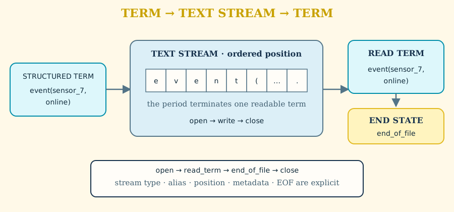
write_event(Path, Event) :-
  setup_call_cleanup(
    open(Path, write, Stream, [type(text)]),
    ( write_canonical(Stream, Event),
      put_char(Stream, '.'),
      nl(Stream)
    ),
    close(Stream)
  ).
In normal mode, setup_call_cleanup/3 is the preferred lifecycle boundary for
resources such as streams: close(Stream) still runs if the protected work
fails, throws, is cut, or its remaining alternatives are abandoned. Strict ISO
mode does not provide this EyeProlog extension.
The period is essential when another Prolog processor will read the result as
a term. write/1-2 uses readable conventional syntax, writeq/1-2 quotes
where needed, and write_canonical/1-2 exposes canonical structure. Dotted
graphic atoms do not need quotes merely because they contain a period:
writeq(./*), writeq(.*), and writeq(...*) output ./*, .*, and ...*
respectively. ISO term output uses only the separator characters needed by the
syntax, so functional arguments, list elements, and operator applications are
emitted compactly when no lexical ambiguity would arise. For example,
writeq([a,b]) outputs [a,b] and writeq(1+2) outputs 1+2; a separator is
still retained where adjacent graphic tokens would otherwise merge, as in
a+ -b.
write_term/2-3 supports quoted/1, ignore_ops/1, numbervars/1, and
variable_names/1. Normal mode additionally accepts the EyeProlog extension
double_quotes(true|false): true lets eligible character/code lists use the
current double_quotes representation. Proper character/code lists can therefore be written
as "text". A proper list whose final segment contains at least two characters/codes
uses that representation for the suffix, so [A,b,c,d,e,f] is written as
[A|"bcdef"]. A partial list such as [a,b|Tail] is written as "ab"||Tail.
This representation choice is independent of ignore_ops/1: with
ignore_ops(true), operator terms use functional notation while an explicitly
requested character/code list remains double quoted. Thus
write_term(f("ab",a+b),[quoted(true),ignore_ops(true),double_quotes(true)])
emits f("ab",+(a,b)). Reversing the two options has the same effect. Strict
ISO mode rejects this implementation-specific write option. Normal mode also accepts the
implementation-specific boolean spacing(true|false) option: false emits
only separators required to avoid lexical ambiguity, while true adds
conventional layout around operators. For example,
write_term(1+1,[spacing(false)]) emits 1+1 and
write_term(1+1,[spacing(true)]) emits 1 + 1. The REPL always follows
the minimal-separator rule, so X=1*1 is displayed as X = 1*1, while a
separator is retained in X = a+ -b because the adjacent graphic tokens would
otherwise merge. Strict ISO mode rejects both extension options.
Character operations are get_char, peek_char, put_char, get_code,
peek_code, and put_code; byte streams use the corresponding byte
predicates. Peeking does not advance the position. Mixing byte operations with
a text stream, or text operations with a binary stream, raises a permission
error rather than guessing an encoding.
read/1-2 reads the next term. read_term/2-3 can also return all variables,
source variable names, and singletons. The metadata contains variables, so a
program normally validates or transforms it before placing it in a ground
query answer. Every read operation creates a fresh variable set: a source name
such as X in two separately read terms does not alias either the caller’s X
or the variable named X by the other read. Within one read term, repeated
occurrences and the variables returned through its metadata still share as
written. stream_property/2 exposes mode, type, alias, position, and
end state. current_input/1, current_output/1, set_input/1, and
set_output/1 manage defaults shared by nested goals.
End of file is a state transition, not merely a character. With
eof_action(eof_code), term input yields end_of_file, character input yields
end_of_file, and code or byte input yields -1; at_end_of_stream/1
tests the position. Repeated input after the end follows the selected
eof_action.
iso-term-io.pl
writes a temporary fixture, reads its terms in order, checks variable metadata,
and observes end of stream. The file lives under /tmp; running the example
does not modify the checkout.
Checkpoint. Write a term round trip and name where quoting, the terminating period, stream type, and close operation matter. Explain why a stream side effect belongs outside the central relation that decides what the term means.
Part VIII summary
The supported ISO facilities make EyeProlog suitable for more than closed rule files:
- control predicates delimit choices and exception recovery;
- collectors distinguish flat, grouped, and canonicalized answer sets;
- reflective predicates treat term structure as data;
- atomic conversions provide standard lexical boundaries;
- dynamic predicates and directives manage explicit solver-local state;
- operators change notation while preserving ordinary term structure; and
- streams connect terms to ordered text or binary I/O.
Chapters 38–40 state the supported profile, list every registered predicate, and document the command line; the conformance corpus fixes success, failure, mode, and error behavior. Use this part for working practice and those chapters for exact reference.
Historical note: the practical language becomes portable
By the late 1970s and 1980s, Prolog had spread from its Marseille origins into several implementation traditions. The Edinburgh and DECsystem-10 lineage in particular helped establish a practical programming vocabulary around ordered control, term inspection, dynamic clauses, operators, and streams. These facilities made Prolog useful far beyond theorem-proving examples, but differences between systems also made portability a recurring concern.
ISO/IEC 13211-1:1995 gave that accumulated practice a common core. It did not freeze the language: constraints, modules, tabling, coroutining, and other facilities continued to develop in implementations and later standardization work. What the standard supplied was a stable shared account of ordinary Prolog terms, control, state, errors, and I/O against which extensions could be named.
Part IX — Reference as practice
Reference is useful only when the route into it is clear. Begin with the task in hand: Chapter 38 answers what source means, Chapter 39 helps select a predicate, and Chapter 40 turns a file into observable evidence. Chapters 41–43 then support study design, boundary decisions, and precise vocabulary. The long catalogs are meant to be entered locally, not memorized linearly.
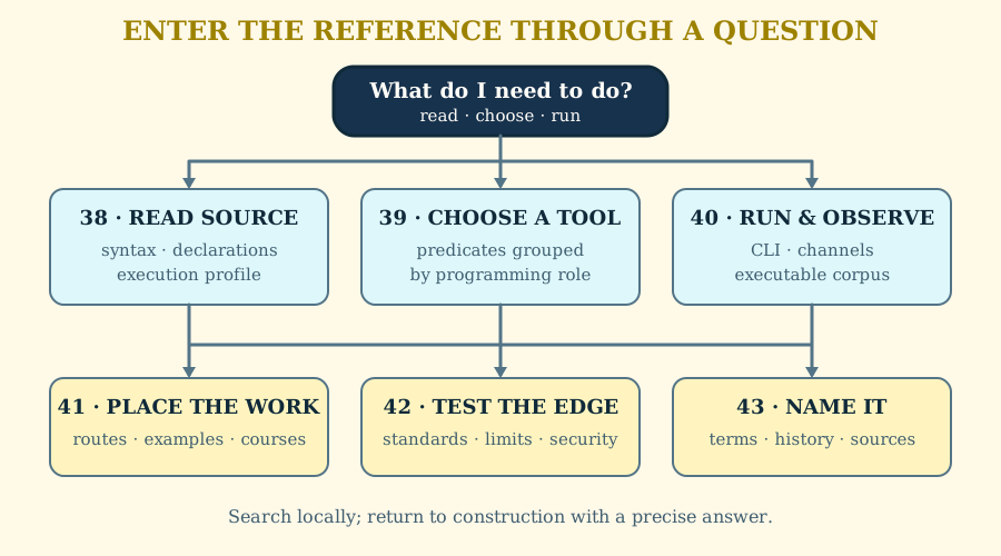
38. Language and ISO profile
The normative strict-core baseline is ISO/IEC 13211-1:1995, as corrected by
Technical Corrigenda 1:2007, 2:2012, and 3:2017. The post-N289 WG17/STC
working draft is used as defect-discovery input, not as an unpublished fourth
Corrigendum. The 2026-08-23 draft through items #73-#76 is tracked by
test/conformance/STC-DRAFT-STATUS.md; where a proposal changes published
semantics, such as #75’s conditional power-underflow proposal, strict mode keeps
the licensed baseline until the change is standardized or explicitly adopted as
a compatibility extension. Normal EyeProlog additionally provides a practical
module interface aligned with later WG17 module amendment work and a
definite-clause-grammar profile following ISO/IEC TS 13211-3. The requirements
clarified by the 2013 Part 2 amendment have a dedicated executable coverage
ledger; the unchanged remainder of Part 2 and the Part 3 profile are documented
and tested compatibility surfaces rather than complete clause-by-clause
certifications.
Normal-mode Prolog source accepted by EyeProlog is UTF-8. % starts a line
comment and /* ... */ delimits a block comment. Plain atoms begin with a
lowercase ASCII letter. Variables begin with uppercase or underscore. The bare
_ is fresh each time. Single quotes delimit quoted atoms; double quotes use
ISO double-quoted-list notation. Integers, decimals, scientific notation,
binary/octal/hexadecimal integers, and character-code constants are accepted.
Normal mode additionally accepts digit-separated integer constants such as
1_000 and 0xCA_FE, with optional layout after the underscore, and the
Trealla-compatible "text"||Tail right-splice for double-quoted chars/codes
lists; strict ISO mode accepts neither syntax extension.
The processor character set is shared by normal and --iso-strict modes because
Part 1 makes it implementation defined rather than an extension boundary.
EyeProlog’s PCS (processor character set) is the Unicode scalar repertoire. Printable ASCII keeps the Part
1 lexical classes; Unicode letters extend alphanumeric name syntax, Unicode
white-space characters are layout, and remaining non-ASCII symbols/punctuation
are extended graphic characters. Character-code and collation values are the
corresponding Unicode scalar integers. Quoting remains available for any atom
spelling that should not depend on an extended lexical class:
:- use_module(library(lists)).

city('München').
message("café").
Inside a quoted atom, a single quote is doubled: 'don''t'. EyeProlog follows
the ISO quoted-character grammar rather than accepting arbitrary backslash
escapes. The symbolic control escapes are \a, \b, \r, \f, \t,
\n, and \v; the meta characters backslash, single quote, double quote, and
back quote may be escaped after a backslash; and numeric octal or hexadecimal
escapes are terminated by a backslash. For example, '\7\' and '\x7\'
both denote the alert character. Forms such as \c, \d, \e, \u, \.
and \ are not ISO quoted-character escapes and are syntax errors.
A literal layout character other than ordinary space is not a quoted
character. In particular, a literal tab or newline inside quotes is a syntax
error. A quoted token can cross a line boundary only through a continuation
escape: a backslash immediately followed by the newline, which contributes no
character to the atom. The NUL character is written readably as '\0\';
digits 8 and 9 are not octal digits, so forms such as '\8\' are syntax
errors. writeq/1 uses octal escapes for other non-symbolic control characters,
for example ESC is written as '\33\'. Double-quoted lists use the same
quoted-character rules. Whitespace is insignificant between tokens, and a %
comment continues to the end of its line. Doubling the active delimiter is
also accepted inside either quoted form, so "" inside double-quoted notation
denotes one literal double quote character.
Graphic tokens use the characters #$&*+-./<=>?@^~\; ! and ; are solo
atoms. A colon is the Part 2 module qualification operator in Module:Goal;
normal mode predeclares it, while --iso-strict does not include it in the
Part 1 initial operator table. Quote an atom whose name itself contains a colon.
Unquoted angle-bracket IRIs are not syntax.
A /* sequence opens a block comment only when it begins a token; inside a
maximal graphic token the slash and star remain atom characters. Graphic tokens
are formed maximally before a period can be recognized as the terminating full
stop. Consequently, interactive input *. or ./*. is not yet a complete term:
the period is part of the graphic atom and the reader waits for a separate
terminating full stop. Thus ./*. . reads the atom ./*. and consumes the
second period as the terminator.
In the grammar below, { x } means zero or more repetitions of x, [ x ]
means that x is optional, and parentheses group alternatives. These marks
describe the grammar; they are not characters written in EyeProlog source.
program             ::= { clause }
clause              ::= head "."
                      | head ":-" goal-list "."
head                ::= term
goal-list           ::= term { "," term }
term                ::= variable | atom-constant | double-quoted-list | number
                      | compound | list | curly-term | parenthesized-term
compound            ::= atom-constant "(" term { "," term } ")"
list                ::= "[" "]"
                      | "[" term { "," term } [ "|" term ] "]"
double-quoted-list  ::= '"' { quoted-character } '"'
curly-term          ::= "{}" | "{" term "}"
parenthesized-term  ::= "(" term [ "," term { "," term } ] ")"
variable            ::= "_"
                      | variable-start { name-continue }
atom-constant       ::= plain-atom | quoted-atom | graphic-atom
plain-atom          ::= lowercase-letter { name-continue }
number              ::= [ "-" ] digits [ "." digits ] [ exponent ]
exponent            ::= ( "e" | "E" ) [ "+" | "-" ] digits
variable-start      ::= uppercase-letter | "_"
name-continue       ::= uppercase-letter | lowercase-letter | digit | "_"
Zero-arity compounds such as ready() are unsupported; use ready. Every
clause ends in a period. The grammar above gives the canonical term shapes.
The initial operator table contains the following ISO-style operators, all
lowered to ordinary compound terms:
- prefix: ISO
?-,\+, unary+, unary-, and\; - control:
,,;, and->; - normal Part 2 module profile:
:at priority 600 (xfy) andmeta_predicateat priority 1150 (fx) so the amendment’s directive spelling such as:- meta_predicate run(:).parses directly; these are not predeclared by--iso-strict; - quad syntax extension:
?-is also a priority-1200xfxoperator so a label may precede a quad query; - grammar rules:
-->and the Part 3 alternative|; - unification and comparison:
=,\=,==,\==,@<,@=<,@>,@>=,is,=:=,=\=,<,=<,>, and>=; - arithmetic:
+,-,*,/,//,div,mod,rem,/\,\/,<<,>>,**, and^.
op/3 directives and runtime calls define or remove prefix, infix, and postfix
operators using the ISO fx, fy, xf, yf, xfx, xfy, and yfx
specifier classes. Variables cannot occur in functor or predicate position.
Parentheses around one term
denote that term; parentheses around two or more comma-separated terms
construct a right-associated ','/2 term. In goal position it is conjunction;
in data position it remains inspectable data.
The pure definite-clause fragment has a Herbrand reading: ground terms denote themselves, predicates denote sets of ground atomic formulas, variables have clause scope, and unification is structural. The implementation performs first-order finite-tree unification with an occurs check. An attempt to bind a variable to a term containing that same variable fails.
An atom constant such as pat is a term. An atomic formula such as
parent(pat, jan) is a proposition that may be a fact, rule head, or goal.
The same surface form, parent(pat, jan), may also be compound data when nested inside
another term; its role comes from context. Predicate identity includes arity,
so edge/2 and edge/3 are different predicates.
Execution is goal-directed rather than complete bottom-up saturation. Goals in
a body normally run from left to right; the solver may select a ready
deterministic built-in early as a pure filter. Ordinary user-defined calls,
including recursive calls, use depth-first resolution unless the source
explicitly declares :- table p/n.. \+/1 is negation as failure, not
classical negation; the separate tnot/1 extension provides well-founded
semantics for eligible finite Datalog components.
EyeProlog supports cut, operator declarations, dynamic database updates, grouped
solutions, exceptions, flags, initialization and inclusion directives, and
standard stream and term I/O. Normal mode additionally provides lifecycle-aware
call_cleanup/2 and setup_call_cleanup/3; these cleanup controls are
EyeProlog extensions and are excluded by --iso-strict. Normal mode also
adds the documented module compatibility surface and a Part 3-oriented DCG
profile.
Module compatibility profile
A module gives predicate identity one more component: module name, predicate name, and arity. The first directive in a module source names the module and lists its public predicates:
% colors.pl
:- module(colors, [tone/1]).

tone(blue).
hidden(module_private).
Another source can import all exports or select particular indicators. An unqualified call first uses a predicate local to the calling module and then an import; a local definition therefore stays distinct from a same-named private predicate elsewhere.
:- use_module('colors.pl', [tone/1]).

hidden(user_local).
answer(Tone, Hidden) :- tone(Tone), hidden(Hidden).
qualified(ok) :- colors:tone(blue).
Imports such as use_module(library(lists)) and
use_module(library(strings)) resolve the bundled modules in Node and the
browser. Atom source designations such as
'colors.pl' resolve relative to the importing file in Node. use_module/1
imports every export; use_module/2 imports only its indicator list, including
an empty list when only qualified calls are wanted. Module:Goal selects a
module explicitly. Repeated module loads are idempotent, while conflicting
imports and requests for predicates that a module does not export are errors.
Part 3-oriented definite clause grammars
A grammar rule Head --> Body. is prepared as an ordinary predicate with two
additional difference-list arguments. Parameterized nonterminals retain their
written arguments, so token(Type)//1 is implemented by token/3.
Nonterminal indicators can be exported and imported through modules:
:- module(vocabulary, [word//1]).

word(noun) --> [robot] | [scientist].
The supported grammar constructs include terminal lists, [], sequencing with
comma, alternatives with ; or |, if-then-else, embedded goals {Goal},
call//1, phrase//1, and !//0. Semicontexts provide look-ahead by restoring
terminals to the remaining sequence:
look_ahead(X), [X] --> [X].
phrase(+Body,?Sequence) accepts or generates a complete sequence.
phrase(+Body,?Sequence,?Rest) leaves Rest unconsumed and is steadfast in
that argument. A variable body raises instantiation_error; a non-callable
body raises type_error(callable). EyeProlog elects to perform the optional
terminal-sequence checks of the ISO/IEC TS 13211-3 working draft, 8.18.1.3 g and h.
It consistently reports type_error(list, Culprit) for invalid input in both
arities and invalid remainder in phrase/3, including improper lists.
Variables, proper lists, and partial lists pass these checks. Validation
precedes grammar execution; an otherwise valid failing grammar does not
suppress the diagnostic. Dedicated regressions enforce this policy separately
from the portable quads, which accept both checking and non-checking outcomes. See
ISO-PART3.md, which also records that the
2023-08-14 working draft specifies type_error(terminal_sequence, Culprit) for
this condition.
A bidirectional expression grammar
DCGs become more useful when the grammar produces a structured term rather than
merely accepting a token list. The checked
dcg-expression-language.pl
example implements a small arithmetic language in both directions. Its parser
respects precedence and left associativity while constructing an abstract syntax
tree:
expression(AST) -->
  term(First),
  additive_tail(First, AST).

additive_tail(Left, AST) -->
  ['+'], term(Right),
  { Next = add(Left, Right) },
  additive_tail(Next, AST).
additive_tail(AST, AST) --> [].
The accumulator removes left recursion without moving parsing into JavaScript.
A second DCG walks the AST in the other direction and emits only the parentheses
needed to preserve its structure. The example therefore exercises parsing,
semantic actions, nonterminal-to-nonterminal state hand-off, generation,
backtracking, phrase/3 remainder handling, and AST-to-token-to-AST
round-tripping. The checked answers are in
examples/output/dcg-expression-language.pl.
Deep sequence hand-off
library(dcgs) provides the common ... //0 helper, which describes an
arbitrary number of input elements. It is not part of ISO Part 3, but it is a
useful interoperability and stress-test relation. A compact hand-off test is:
a --> ..., epsilon.
epsilon --> [].
Here the remaining sequence is repeatedly passed from ... //0 to another
nonterminal. For a finite compact list, EyeProlog can scan the arbitrary
sequence iteratively instead of consuming one ordinary solver depth level per
list cell. If the continuation is structurally proven to be a zero-width
identity grammar such as epsilon//0, the hand-off can be continued without
constructing a fresh general clause-resolution frame at every suffix. The list
spine is still traversed; this is a control/allocation optimization rather than
an O(1) semantic shortcut.
The optimization is deliberately narrow. phrase(..., Sequence, Rest) still
enumerates the valid remainders, open or non-compact inputs retain ordinary
relational behavior, and grammars that can consume or constrain the remainder
are not treated as identity continuations. time/1 can be used in normal mode
to measure such runs; its inference counter records solver-level inferences and
does not count every internal step of an optimized scanner.
Part 3 leaves \+//1 and standalone ->//2 implementation dependent.
EyeProlog uses non-consuming negation (\+ Body tests from the current state)
and threads the state produced by the condition into the then-grammar.
Directives and protected built-ins
false/0 is the ISO always-failing built-in. It is protected as a static
procedure, so source clauses headed by false are rejected instead of being
interpreted as directives or integrity constraints.
Standard directives include dynamic/1, multifile/1, discontiguous/1,
op/3, char_conversion/2, initialization/1, include/1,
ensure_loaded/1, module/2, use_module/1, use_module/2,
meta_predicate/1, and set_prolog_flag/2. Initialization goals run once
after program preparation and before host queries. Included text is expanded
in place; repeated ensure_loaded/1 designations are loaded once.
Normal output contains only ground query answers, one term and period at a time. Source facts are not echoed as new conclusions, and duplicate answers are suppressed. Answers are not asserted back into the running program. Supported output syntax is designed to be readable as Prolog input accepted by EyeProlog.
Explicit tabling and recursion planning
The program loader analyzes predicate dependencies and recursion so the solver
can choose semantics-preserving indexes and fast paths. That analysis does
not decide whether a predicate is tabled. Ordinary predicates—including
recursive ones—use indexed, depth-first Prolog resolution unless their source
explicitly declares :- table p/n..
An explicitly tabled positive recursive predicate is coordinated through an answer table: recurring calls consume answers already found, new answers are recorded, and evaluation continues toward a fixed point. For eligible large, finite, function-free Datalog components, EyeProlog may represent that declared table as one shared most-general relation or an indexed least model. For other declared tables the engine may infer structurally bound input positions to improve table reuse. These are implementation choices inside an explicit table declaration; they never opt an undeclared predicate into tabling.
Ordinary \+/1 remains ISO-style negation as failure. The separate tnot/1
extension explicitly requests well-founded evaluation for eligible finite,
range-restricted Datalog dependencies. wfs_truth/2 reports the three-valued
state of a ground callable as true, false, or undefined. Strict ISO mode
exposes none of table, tnot/1, or wfs_truth/2.
Query execution
The host-supplied goal must be callable and may contain constants or variables.
An unbound goal raises instantiation_error; a non-callable goal raises
type_error(callable). A program without a supplied goal prints no normal
answers. The host:
- parses all inputs into one program;
- collects source facts and host-supplied goals;
- runs initialization goals;
- solves each supplied goal;
- retains only ground answers;
- removes answers identical to source facts and suppresses duplicates;
- prints each answer and, only when requested, its
why/2explanation.
Goal selection affects host execution rather than the program’s logical meaning. One goal’s answers are not asserted for later goals, although explicitly declared tables may be reused during the solver run. For stable output, queries for known predicates are grouped by the source order in which their predicate groups first appear; goals within one group retain their supplied order. Queries for predicates with no group follow the known groups.
39. Predicate reference
EyeProlog’s normal predicate surface has two layers: 129 core registry indicators and 404 distinct non-ISO library or normal-extension indicators. Because phrase/2 and phrase/3 occur in both layers, their union contains 533 distinct predicate indicators.
Core predicates are available without a library import. Bundled libraries add reusable relations for collections, constraints, graphs, text, time, cryptography, files, and other domains. Interoperability notes identify the subset shared with Trealla and Scryer, and the complete alphabetical reference gives one compact contract for every indicator.
Notation and conventions
The call patterns below use + for an argument that must be sufficiently
instantiated, - for a result normally produced by the call, and ? for an
argument that may be supplied or returned. These are principal operational
modes, not a separate mode system enforced by the parser. A call described as
semidet succeeds at most once; a nondet call may yield further answers on
backtracking. Unless stated otherwise, checking a result that does not unify
simply fails.
Built-in dispatch is authoritative and built-in procedures cannot be modified
through the dynamic database predicates. Source clauses with the same indicator
do not replace a built-in implementation. clause/2 and op/3 are the two
dispatch exceptions: when a program defines a source predicate with that same
indicator, EyeProlog uses the source clauses. false/0 is stricter still and is
rejected as a source-clause head. Portable programs should avoid every such
collision because other Prolog systems commonly reject it while loading.
Core registry
EyeProlog’s default registry contains the built-ins in its ISO compatibility
profile. Where ISO/IEC 13211-1:1995 defines a predicate, EyeProlog uses its
standard predicate indicator; the registry also includes the later or common
compatibility predicates identified below. Arithmetic is expressed through
is/2 rather than output arguments on arithmetic predicates. The registry
contains 129 name/arity entries across 100 names.
Core registry at a glance
- Control and exceptions —
true/0,fail/0,false/0,!/0,call/1,call/2,call/3,call/4,call/5,call/6,call/7,call/8,\+/1,once/1,repeat/0,;/2,->/2,catch/3,throw/1,halt/0,halt/1 - Unification and identity —
=/2,unify_with_occurs_check/2,\=/2,subsumes_term/2,==/2,\==/2 - Type tests —
var/1,nonvar/1,atom/1,integer/1,float/1,number/1,atomic/1,compound/1,callable/1,ground/1,acyclic_term/1 - Term order —
compare/3,@</2,@=</2,@>/2,@>=/2,sort/2,keysort/2 - Term inspection —
functor/3,arg/3,=../2,copy_term/2,term_variables/2 - Collection —
findall/3,bagof/3,setof/3 - Grammar processing —
phrase/2,phrase/3 - Database and information —
clause/2,asserta/1,assertz/1,retract/1,retractall/1,abolish/1,current_predicate/1 - Operators, conversion, and flags —
op/3,current_op/3,char_conversion/2,current_char_conversion/2,current_prolog_flag/2,set_prolog_flag/2 - Atomic terms —
atom_length/2,atom_concat/3,sub_atom/5,atom_chars/2,atom_codes/2,char_code/2,number_chars/2,number_codes/2 - Stream control —
open/3,open/4,close/1,close/2,current_input/1,current_output/1,set_input/1,set_output/1,flush_output/0,flush_output/1,stream_property/2,set_stream_position/2,at_end_of_stream/0,at_end_of_stream/1 - Character input —
get_char/1,get_char/2,peek_char/1,peek_char/2,get_code/1,get_code/2,peek_code/1,peek_code/2 - Character output —
put_char/1,put_char/2,put_code/1,put_code/2,nl/0,nl/1 - Byte input/output —
get_byte/1,get_byte/2,peek_byte/1,peek_byte/2,put_byte/1,put_byte/2 - Term input —
read/1,read/2,read_term/2,read_term/3 - Term output —
write/1,write/2,writeq/1,writeq/2,write_canonical/1,write_canonical/2,write_term/2,write_term/3 - Arithmetic —
is/2,=:=/2,=\=/2,</2,=</2,>/2,>=/2
Control, search, and exceptions
true— Succeeds once without binding variables.fail,false— Always fail.false/0is provided as a compatibility alias and is also forbidden as a source-clause head.!— Commits to choices made since entry into the current predicate invocation. It does not erase alternatives belonging to an enclosing caller.call(+Goal)— Calls an atom or compound goal. An unbound argument raises instantiation_error; another non-callable term raises type_error(callable).call(+Closure,?Arg,...)—call/2throughcall/8append their extra arguments to an atom or compound closure, as specified by Corrigendum 2.\+(+Goal)— Negation as finite failure. It succeeds once whenGoalhas no solution and never exports bindings made while testingGoal. Bind variables needed by the test first.once(+Goal)— Returns only the first solution ofGoal, or fails when there is none.repeat— Produces an unbounded sequence of successes; normally paired with a test, cut, exception, orhalt/0.Left ; Right— EnumeratesLeft, thenRight, restoring the incoming environment between branches. A cut inside a called predicate cannot discard the other branch.If -> Then— Commits to the first solution ofIfand runsThen; it does not provide an else branch by itself.(If -> Then ; Else)— RunsThenfrom the first solution ofIf, otherwise runsElse. Alternatives ofIfare discarded.catch(+Goal,?Catcher,+Recovery)— RunsGoal; on a matching thrown ball orPrologError, unifies it withCatcherand callsRecovery. Runtime errors are exposed as error(Formal,eyeprolog).throw(+Ball)— Throws a copied nonvariable term. An unbound ball raisesinstantiation_error.halt,halt(+Status)— Stops the processor with status0or the supplied integer. The JavaScript API reports the status without terminating its host process.
;/2 recognizes an ->/2 term on its left and implements the ISO
if-then-else commitment described above. Cuts and committed conditions are
operational controls; use ordinary relations when all alternatives should
remain observable.
Definite clause grammar processing
phrase(+Body,?Sequence)— Parses or generatesSequencewith a Part 3 grammar body and requires complete consumption.phrase(+Body,?Sequence,?Rest)— Parses or generates a prefix described byBodyand unifiesRestwith the unconsumed terminal sequence. The final unification is delayed so the third argument is steadfast.
Grammar rules are expanded during program preparation and therefore appear to
the solver as ordinary predicates with two extra arguments. Dynamic grammar
bodies passed to phrase/2-3 use the same expansion rules. This includes
module qualification and the caller module used by embedded or meta-called
nonterminals.
Unification, type tests, and term order
?Left = ?Right— Unifies two terms and returns the resulting bindings. EyeProlog rejects direct and indirect cyclic bindings.unify_with_occurs_check(?Left,?Right)— Performs occurs-check-safe unification. Because ordinary EyeProlog unification is already cycle-safe, it has the same successful bindings as=/2.?Left \= ?Right— Succeeds only when the terms cannot unify at call time. It is a test, not a delayed disequality constraint.subsumes_term(+General,+Specific)— Tests one-sided syntactic unification without binding either argument. Variables inSpecificremain unchanged.?Left == ?Right,?Left \== ?Right— Test term identity or non-identity without binding variables. Two distinct unbound variables are not identical.var(?Term),nonvar(?Term)— Test whether the dereferenced term is or is not an unbound variable.atom(?Term),integer(?Term),float(?Term),number(?Term)— Test the corresponding scalar category. Integer values retain arbitrary precision; finite noninteger numeric values are floats.atomic(?Term),compound(?Term),callable(?Term),ground(?Term),acyclic_term(?Term)— Test for an ISO atomic term, a compound, a callable atom/compound, a term containing no unbound variables, or a finite acyclic term. A default double-quoted value is a list and is therefore compound unless it is empty.compare(?Order,+Left,+Right)— UnifiesOrderwith<,=, or>according to standard term order. A supplied order must be one of those atoms.Left @< Right,Left @=< Right,Left @> Right,Left @>= Right— Compare terms without arithmetic evaluation or bindings. These calls are semidet.sort(+List,?Sorted)— Sorts by standard term order and removes identical duplicates.keysort(+Pairs,?Sorted)— Stably sortsKey-Valuepairs by key without removing duplicates.
For ISO terms, the standard term order is variables, numbers, atoms, then compounds;
compound terms compare by arity, functor, and arguments. Within the numeric
category, floats precede integers; floats compare by finite numeric value and
integers compare exactly. ISO leaves the ordering of two distinct variables
implementation dependent, subject to stability while a sorted list is being
created. EyeProlog assigns a creation ordinal to each logical variable and
carries that ordinal on the variable term itself; repeated occurrences share it
within parsing or clause-freshening scope. It therefore does not keep a
process-global table of every fresh variable name ever created, so long-running
generators can create and discard fresh variables without growing an unrelated
host Map. Double-quoted Prolog source
follows the double_quotes flag and never creates an extra host-only scalar
category.
Term construction and inspection
functor(+Term,?Name,?Arity)— Decomposes a term. Scalars have arity zero.functor(-Term,+Name,+Arity)— Constructs a scalar whenArityis zero or a compound with fresh arguments otherwise. Arity must be a nonnegative representable integer and a positive-arity name must be an atom.arg(+Index,+Term,?Argument)— Selects the one-based argument of a compound. Index zero or an index beyond the arity fails; a negative index is a domain error.?Term =.. ?List— Converts a term to[Functor\|Arguments]or constructs a term from a nonempty proper list. A one-item list constructs its atomic item.copy_term(+Term,-Copy)— Copies the dereferenced term while replacing every distinct unbound variable with a fresh variable and preserving variable sharing.term_variables(+Term,?Variables)— Returns distinct variables in first-occurrence traversal order. A supplied result may be a proper or partial list.
Construction calls raise instantiation_error when neither side supplies the
required shape. =../2 distinguishes an incomplete list
(instantiation_error) from an improper list (type_error(list)).
Solution collection
findall(+Template,+Goal,?Bag)— Collects a fresh copy ofTemplatefor every solution ofGoal, preserving solution order. It succeeds with[]when there are no solutions and treats all free variables existentially.bagof(+Template,+Goal,?Bag)— Groups answers by free variables not present inTemplate. It yields one nonempty bag per witness group and fails when no group exists. Prefix variables with^inGoalto quantify them existentially.setof(+Template,+Goal,?Set)— Has the grouping behavior ofbagof/3, then sorts each group by profile term order and removes identical duplicates.
Each collector runs its goal in an isolated inner search while sharing the current logical program and stream state. Collected terms are copied, so local variables do not escape accidentally. The bag argument must be a proper or partial list.
Dynamic database and procedure information
clause(+Head,?Body)— Enumerates fresh copies of source clauses matching the callableHead; facts have bodytrue. Only public procedures can be inspected: a procedure defined by a Prolog text is static unless a dynamic/1 directive declares it, and a procedure first created by assertz/1 or asserta/1 is dynamic. Access to a static user procedure, or to a built-in, raises permission_error(access,private_procedure). This applies in every execution mode, not only under--iso-strict, and matches the permission_error(modify,static_procedure) that assertz/1 and retract/1 already raise for the same procedures. Normal mode additionally accepts a public/1 directive and adefault_procedure_accessflag that open static procedures to inspection; see below.asserta(+Clause),assertz(+Clause)— Insert a copied fact or rule at the beginning or end of a predicate declared dynamic/1. Static and built-in procedures cannot be modified.retract(+Clause)— Removes matching dynamic clauses one at a time on backtracking. A call sees the logical update view captured when it began. A fact pattern matches facts only.retractall(+Head)— Removes every matching clause from a dynamic procedure, succeeds when none match, and keeps the empty dynamic procedure known.abolish(+Name/+Arity)— Removes a dynamic procedure and its clauses. The indicator must contain an atom and a nonnegative representable integer.current_predicate(?Name/?Arity)— Enumerates predicate groups present in the loaded program, including empty dynamic groups. It does not enumerate registry-only built-ins.
Declare mutable predicates explicitly, including empty ones:
:- dynamic(cache/2).

remember(Key, Value) :- retract(cache(Key, _)), !, assertz(cache(Key, Value)).
remember(Key, Value) :- assertz(cache(Key, Value)).
Assertions and retractions invalidate affected reasoning tables. Mutating a predicate that was not declared dynamic raises a permission error rather than silently changing a static program.
Operators, character conversion, and flags
op(+Priority,+Specifier,+NameOrNames)— Defines or removes operators in the current program. Priority is0..1200; specifiers arefx,fy,xf,yf,xfx,xfy, oryfx; names may be one atom or a proper list. Priority zero removes the definition.,and\|cannot be modified.current_op(?Priority,?Specifier,?Name)— Enumerates active operator definitions and filters supplied arguments.char_conversion(+Input,+Output)— Installs a one-character conversion. In prepared Prolog text, later unquoted characters are converted whenchar_conversion=on; quoted characters are unchanged. The same mapping initializes execution-time term input. Mapping a character to itself removes its custom mapping.current_char_conversion(?Input,?Output)— Enumerates installed nonidentity conversions.current_prolog_flag(?Flag,?Value)— Enumerates flags or retrieves one named flag. An unknown bound flag raises domain_error(prolog_flag).-
set_prolog_flag(+Flag,+Value)— Changes a supported mutable flag after validating its allowed atom value. Read-only flags raise a permission error. bounded— Default:false; Allowed:false; Mutable: no.integer_rounding_function— Default:toward_zero; Allowed:toward_zero; Mutable: no.char_conversion— Default:on; Allowed:on,off; Mutable: yes.debug— Default:off; Allowed:on,off; Mutable: yes.max_integer— Default: no current value becausebounded=false; Allowed: not applicable; Mutable: no.min_integer— Default: no current value becausebounded=false; Allowed: not applicable; Mutable: no.max_arity— Default:unbounded; Allowed:unbounded; Mutable: no.unknown— Default:error; Allowed:error,fail,warning; Mutable: yes.double_quotes— Default:chars; Allowed:chars,codes,atom; Mutable: yes.occurs_check— Default:true; Allowed:true,error; Mutable: yes.
Because bounded=false, current_prolog_flag(max_integer, _) and
current_prolog_flag(min_integer, _) fail, and EyeProlog does not expose an
unbounded sentinel as either flag value. This is a deliberate implementation
choice rather than a requirement: ISO 7.11.1.1 defines the bounded flag and
does not govern current_prolog_flag/2 outcomes, and 7.11.1.2 and 7.11.1.3
give max_integer and min_integer an implementation-defined default value
unconditionally, making the bounded condition a constraint on what the value
means rather than on whether the flag exists. A processor with unbounded
integers has no largest integer to report, so EyeProlog declines to invent one.
See conformance-report.md for the alternative reading.
Preparation-time char_conversion/2 mappings affect later unquoted source text
and also initialize the execution-time conversion mapping; setting the
char_conversion flag to off disables conversion for following source text.
Quoted source characters are not converted.
Both normal EyeProlog and strict ISO core mode use the ISO unknown=error
default. Interactive set_prolog_flag/2 changes are retained when the REPL
consults another file or imports a module instead of being reset by the host
rebuild of the program. Programs that intentionally treat an undefined
predicate as failure must opt in with set_prolog_flag(unknown, fail); bundled
examples and non-ISO corpus cases that depend on that policy do so explicitly.
Reading static procedures
A procedure defined by a Prolog text is static, so clause/2 refuses it
(ISO 7.5.2, 7.5.3, 8.8.1.3). Declaring the procedure dynamic lifts the
restriction, but it also makes the procedure modifiable, and for a
meta-interpreter it means annotating a program you may not want to edit and
enumerating every predicate you intend to read.
ISO 7.5.3 has a NOTE observing that a public/1 directive declaring
user-defined procedures to be public would be an extension. Normal EyeProlog
provides it:
:- public(elk/1).

elk(X) :- moose(X).

moose(bertha).
clause(elk(bertha), Body) now succeeds with Body = moose(bertha), while
moose/1 carries no declaration and stays private. A public procedure is still
static: assertz(elk(clara)) continues to raise
permission_error(modify,static_procedure). The directive grants read access
only.
To open every user-defined procedure at once, set the
default_procedure_access flag to public:
:- set_prolog_flag(default_procedure_access, public).

solve(true) :- !.
solve((A, B)) :- !, solve(A), solve(B).
solve(H) :- clause(H, Body), solve(Body).

elk(X) :- moose(X).
moose(bertha).
grazes(X) :- elk(X).
solve(grazes(W)) yields W = bertha without a single declaration on the
interpreted program. The flag changes access, not mutability or existence:
procedures remain static, and built-in procedures remain private, so
clause(atom(_), _) still raises permission_error(access,private_procedure).
The supported values are private (the default, matching ISO) and public.
Both the directive and the flag are extensions, so strict ISO core mode offers
neither: public/1 is rejected as an implementation-specific directive, and
current_prolog_flag(default_procedure_access, _) raises
domain_error(prolog_flag).
The occurs_check flag is an EyeProlog diagnostic
extension rather than an ISO-defined core flag: it is absent in strict mode,
while normal mode keeps its true default and optional error diagnostic for
STO attempts. Operator and flag directives are processed per program rather
than changing global JavaScript state. The double_quotes setting affects
subsequent source text, included files, command-line and API goal text, and
terms read by read_term/*:
% Default: a list of one-character atoms.
chars("ab").                 % chars([a,b])

:- set_prolog_flag(double_quotes, codes).
codes("ab").                 % codes([97,98])

:- set_prolog_flag(double_quotes, atom).
quoted_atom("ab").           % quoted_atom(ab)
Atomic-term operations and conversions
atom_length(+Atom,?Length)— Counts Unicode code points, not UTF-16 code units. A supplied length must be a nonnegative integer.atom_concat(?Prefix,?Suffix,?Whole)— Concatenates two atoms, removes a supplied prefix or suffix, or enumerates every split when onlyWholeis bound. At leastWhole, or both parts, must determine the operation.sub_atom(+Atom,?Before,?Length,?After,?SubAtom)— Enumerates substrings and their Unicode-code-point offsets. Supplied counts must be nonnegative integers.atom_chars(?Atom,?Chars),atom_codes(?Atom,?Codes)— Convert between an atom and a proper list of one-character atoms or character codes. Both profiles use EyeProlog’s Unicode scalar PCS/codes; surrogates and values above U+10FFFF are rejected. At least one side must be instantiated.char_code(?Character,?Code)— Converts one character atom and its collating/code value. Both profiles accept Unicode scalar codes and reject surrogates/out-of-range values.number_chars(?Number,?Chars),number_codes(?Number,?Codes)— Convert finite numbers to canonical text or parse a proper character/code list using number and negative-number syntax, including radix integers, character-code constants, and leading layout. Normal mode also accepts digit separators in integer input; strict mode retains the ISO syntax. The input is not parsed as a general term: grouping such as(0)is a syntax error. At least one side must be instantiated; malformed numeric input raises syntax_error(number).
Conversions accept partial output lists when the atomic input is known, but
constructing an atom or number requires a complete proper list with no unbound
elements. Numeric parsing accepts ISO layout before tokens, including layout between a
minus token and the following numeric token. A single-line %... comment may
therefore follow - directly because % cannot continue a graphic token; an
adjacent bracketed comment in -/**/1 remains a syntax error under the eager
token-consumer rule. Decimal fractions and decimal exponents are supported;
the apostrophe character code is written with a doubled apostrophe as 0'''
and has value 39, while a literal space character code is 0' and has value
- Character-code constants consume one Unicode scalar, including a
non-BMP character. Trailing layout, comments, and other material are rejected;
bound integers are converted to their canonical decimal spelling, and
non-finite values are rejected. Finite floats use the shortest decimal spelling
that round-trips to the same host floating-point value, with an explicit
fractional part so the result remains a Prolog float; for example,
1.0000000000000001is represented as1.0. Equivalent spellings of the same numeric type compare by value, preserving the standard conversion round trip, while integer and floating-point terms remain distinct. The numeric conversion behavior follows the 74 numbered cases in Ulrich Neumerkel’s contemporarynumber_chars/2comparison, including the Corrigendum 2 error-precedence cases;number_codes/2uses the same numeric parser.
Streams and unit I/O
Stream arguments accept an alias atom or the opaque handle returned by
open/3 or open/4. Omitting a stream argument selects the current standard
input or output.
open(+Source,+Mode,-Stream),open(+Source,+Mode,-Stream,+Options)— Opens an atom path inread,write, orappendmode. Options are type(text or binary), alias(Atom), reposition(true or false), and eof_action(error, eof_code, or reset).close(+Stream),close(+Stream,+Options)— Closes a nonstandard stream. The only close option is force(true or false); standard streams remain available.current_input(?Stream),current_output(?Stream)— Return or test the current input or output handle.set_input(+Stream),set_output(+Stream)— Select an existing stream with the required direction.flush_output,flush_output(+Stream)— Completes successfully for the current output or validates and flushes the selected output stream. EyeProlog writes synchronously.stream_property(?Stream,?Property)— Enumerates streams and their properties: mode/1, type/1, reposition/1, eof_action/1, position/1, input, output, end_of_stream/1, and optional alias/1 and file_name/1.set_stream_position(+Stream,+Position)— Repositions a stream opened with reposition(true).Positionis a nonnegative integer or position(Integer) within the stream content.at_end_of_stream,at_end_of_stream(+Stream)— Succeeds when the current or selected input position is at or beyond its content.get_char(?Character),get_char(+Stream,?Character)— Reads one text character; end of input isend_of_file.peek_char(?Character),peek_char(+Stream,?Character)— Observes the next text character without advancing.get_code(?Code),get_code(+Stream,?Code)— Reads a character code; end of input is-1. Both profiles return codes from EyeProlog’s Unicode scalar PCS.peek_code(?Code),peek_code(+Stream,?Code)— Observes the next Unicode scalar character code without advancing.get_byte(?Byte),get_byte(+Stream,?Byte)— Reads one unit from a binary stream; end of input is-1.peek_byte(?Byte),peek_byte(+Stream,?Byte)— Observes the next binary unit without advancing.put_char(+Character),put_char(+Stream,+Character)— Writes one character atom to a text stream.put_code(+Code),put_code(+Stream,+Code)— Writes one character code to a text stream. Both profiles accept Unicode scalar codes.put_byte(+Byte),put_byte(+Stream,+Byte)— Writes an integer in0..255to a binary stream.nl,nl(+Stream)— Writes a newline to a text stream.
Text operations on binary streams and byte operations on text streams raise
permission errors. After EOF, eof_action(error) rejects another consuming
read, eof_code continues returning the EOF value, and reset resumes from
the beginning. A peek does not mark the stream as past-end.
Term input and output
read(?Term),read(+Stream,?Term)— Reads one full-stop-terminated Prolog term from a text stream. Returnsend_of_filewhen no term remains.read_term(?Term,+Options),read_term(+Stream,?Term,+Options)— Reads a term and supports variables(List), variable_names(Pairs), and singletons(Pairs). Unknown options raise domain_error(read_option).write(+Term),write(+Stream,+Term)— Writes readable operator notation without quoting atoms merely because quoting would be required for reparsing. Number variables are enabled.writeq(+Term),writeq(+Stream,+Term)— Likewrite, but quotes atoms when required for unambiguous input syntax.write_canonical(+Term),write_canonical(+Stream,+Term)— Writes quoted canonical functor notation while ignoring operators and without interpreting $VAR/1.write_term(+Term,+Options),write_term(+Stream,+Term,+Options)— Writes with quoted(true or false), ignore_ops(true or false), numbervars(true or false), and variable_names([Name=Variable,…]). Normal mode also supports double_quotes(true or false) and spacing(true or false).double_quotes(true)remains effective withignore_ops(true): operator terms are written functionally while eligible character/code lists retain double-quoted notation, independently of option order.
Term input uses the program’s current operator table and the same ISO quoted-character
syntax as source text, including backslash-terminated octal and hexadecimal
escapes such as '\7\' and '\x7\'. This applies equally to read/1-2 and
read_term/2-3. Installed character conversions are applied outside quoted text
when the char_conversion flag is on. variable_names/1 and singletons/1 omit anonymous variables. Output
predicates do not append a period or newline; call write/1, then write('.')
and nl/0 when emitting a complete source term manually.
A standalone numeric term read by read/1-2 or read_term/2-3 uses the same
bounded numeric scanner and canonical value conversion as number_chars/2.
Consequently every numeric character sequence accepted by number_chars/2 has
the same value when read as a full-stop-terminated term, without requiring EOF
after that term.
Arithmetic expressions
is(?Result,+Expression)— EvaluatesExpressiononce and unifies its numeric value withResult. It is evaluation plus unification, not mutable assignment.Left =:= Right,Left =\= Right— Evaluate both sides and test numeric equality or inequality. Integer/float representation differences do not by themselves make values unequal.Left < Right,Left =< Right,Left > Right,Left >= Right— Evaluate both sides and perform the indicated numeric comparison.
Every variable in an arithmetic expression must already be bound to a number or evaluable expression. Integers use arbitrary-precision arithmetic while an operation remains in the integer domain; operations requiring floating point convert their operands to finite JavaScript numbers.
- Literals and constants — Integer and finite floating-point literals;
piandeproduce floating-point constants. - Unary arithmetic — Unary
+, unary-, and integer bitwise complement\. - Basic binary arithmetic —
+,-, and*preserve integers when both operands are integers./produces a float and rejects a zero divisor. - Exponentiation —
Base ^ Exponentremains an integer for nonnegative integer operands. Corrigendum 3 requires a float base for most negative integer exponents;**is floating-point exponentiation. - Integer division —
//anddivrequire integers and reject zero divisors.//rounds toward zero as reported byinteger_rounding_function;divrounds down. - Integer remainder —
remis the truncating remainder;modnormalizes the result with the divisor’s sign. Both require integers and a nonzero divisor. - Bit operations — Integer
/\,\/,xor,<<, and>>, plus unary\. - Numeric normalization —
abs,sign, andfloat. Integerabsandsignpreserve integer results;floatproduces a float. - Rounding —
truncate,round,ceiling, andfloorproduce integers. - Float decomposition —
float_integer_partandfloat_fractional_partrequire a float and return floats. - Min/max and transcendental functions —
min,max,sin,cos,atan,asin,acos,atan2,tan,exp,log, andsqrt;piis the Corrigendum 2 constant.
Arithmetic comparisons evaluate both operands. Standard term-order predicates
(@<, @=<, @>, @>=) compare terms without arithmetic evaluation.
EyeProlog’s documented profile order distinguishes floats from integers rather
than applying arithmetic equality across representations. Double-quoted text
does not introduce another ISO term-order category: it becomes the list or atom
selected by double_quotes before comparison.
Errors
ISO built-ins distinguish logical failure from exceptional calls. Insufficient
instantiation raises instantiation_error; wrong argument categories raise
type_error; invalid values raise domain_error; and arithmetic faults raise
evaluation_error. JavaScript embedders receive these as PrologError
instances whose message contains the corresponding Prolog error term.
- instantiation_error — A required callable, stream, number, list, option value, or construction input is still unbound.
- type_error(Expected,Culprit) — A bound value has the wrong term category, such as a noninteger index or non-callable goal.
- domain_error(Domain,Culprit) — The type is correct but the value is outside the supported domain, such as a bad stream option or operator priority.
- representation_error(Flag) — A value cannot be represented by the profile, such as an invalid Unicode scalar code.
- evaluation_error(zero_divisor) — Integer or floating-point division was attempted with a zero divisor.
- evaluation_error(undefined) — Floating-point evaluation produced a non-finite or undefined result.
- permission_error(Operation,Permission,Culprit) — A static procedure was modified, a stream was used in the wrong mode, or a protected resource was accessed.
- existence_error(Object,Culprit) — A stream, source sink, or required procedure does not exist.
- syntax_error(number), syntax_error(read_term) — Lexical number conversion or streamed term parsing failed.
catch/3 converts a PrologError into a catchable
error(Formal,eyeprolog) term. throw/1 copies its ball before unwinding: bound
parts are preserved, repeated variables remain shared within the copied ball,
and unbound variables are fresh with respect to the protected goal and catcher.
Catchable error terms follow the same variable-freshening rule. The interactive
top level uses the same ISO error envelope for uncaught processor errors, so an
ordinary runtime error is displayed as error(Formal,eyeprolog) rather than
dropping the implementation-defined second argument. Variables that occur in an
uncaught ISO error are rendered with fresh answer names such as _A rather than
reusing query-variable spellings such as X or Xx; this keeps the displayed
error consistent with the copied exception term. An unmatched ball or error
continues outward.
Streams belong to one solver run and are shared by nested calls, exceptions,
and solution collectors. user_input and user_output are always present.
open/4 supports type/1, alias/1, reposition/1, and eof_action/1;
read_term/3 supports variables/1, variable_names/1, and singletons/1.
The JavaScript ioOptions.input and ioOptions.write hooks connect standard
streams to an embedder. File-backed streams use synchronous lifecycle semantics
so side effects occur in Prolog execution order.
Normal-mode extensions
The normal profile also supplies a small number of runtime controls that are not members of the isolated ISO registry. They are kept separate here so the core boundary remains visible.
Cleanup controls
call_cleanup/2 and setup_call_cleanup/3 are normal EyeProlog runtime extensions rather than members of the isolated ISO builtin registry. They protect a goal across deterministic completion, exhaustion, cut, top-level abandonment, and exception unwinding, running Cleanup exactly once. setup_call_cleanup/3 runs Setup once and installs Cleanup only after Setup succeeds. A successful Cleanup run before a deterministic answer contributes its substitutions to that answer. Nested cleanups run inside-out, and strict ISO mode does not provide either predicate.
Bundled libraries
EyeProlog exposes 404 distinct non-ISO library and normal-extension predicate
indicators in addition to the 129 indicators in its isolated ISO profile.
282 are defined entirely as ordinary Prolog clauses in focused modules under
src/lib/; 122 use host support for control, attributed variables,
constraints, character conversion, filesystem/OS access, timing, cryptography,
or observability. The ISO and library catalogs therefore cover 533 distinct predicate indicators. A normal-runtime predicate that is intentionally
re-exported by a compatibility module is counted once in this library surface:
for example call_cleanup/2 and setup_call_cleanup/3 are exported by
library(iso_ext), while time/1 and statistics/2 are available from
library(time). statistics/0, tnot/1, and wfs_truth/2 remain
normal-runtime extensions outside the library catalog. These additions are
absent from the strict ISO registry.
The sources are src/lib/aggregate.pl, src/lib/arithmetic.pl,
src/lib/assoc.pl, src/lib/atts.pl, src/lib/between.pl,
src/lib/charsio.pl, src/lib/clpb.pl, src/lib/clpz.pl,
src/lib/comparison.pl, src/lib/crypto.pl, src/lib/dates.pl, src/lib/dcgs.pl,
src/lib/debug.pl, src/lib/dif.pl, src/lib/error.pl,
src/lib/eyelet.pl, src/lib/files.pl, src/lib/format.pl, src/lib/http.pl,
src/lib/freeze.pl, src/lib/gensym.pl, src/lib/iso_ext.pl, src/lib/json.pl,
src/lib/lambda.pl, src/lib/lists.pl, src/lib/ordsets.pl,
src/lib/os.pl, src/lib/pairs.pl, src/lib/pio.pl, src/lib/primes.pl,
src/lib/prologue.pl, src/lib/random.pl, src/lib/reif.pl, src/lib/si.pl,
src/lib/sockets.pl, src/lib/strings.pl, src/lib/tabling.pl, src/lib/terms.pl,
src/lib/time.pl, src/lib/ugraphs.pl, src/lib/uuid.pl, and
src/lib/when.pl. Each declares a same-named module
with module/2; there is no catch-all library(eyeprolog). A program imports
only the modules it needs, and
use_module/2 can select an even smaller indicator list. The Prologue
module exposes p.p.1 through p.p.11 of the
working-draft Prologue,
as a compatibility facade over the canonical lists, between, iso_ext,
and freeze modules. src/standard-library.js registers the module sources and explicit module-owned host adapters. For example, attributed-variable support lives in
src/atts-host.js, while cryptographic primitives live in src/crypto-host.js. Whenever src/lib/foo.pl needs a private runtime primitive, that
primitive is registered from src/foo-host.js; pure Prolog libraries deliberately
have no host file. This keeps character I/O, filesystem access, crypto, timing,
attributed-variable support, and other runtime bridges with the module that owns
their public semantics instead of in a compatibility grab bag. Private runtime adapters remain owned by the module whose public semantics they support; no shared compatibility grab bag participates in library execution. Explicit use_module/1-2 loads remain supported; outside strict ISO mode, the bundled-library autoloader may also load the canonical owner of any exported src/lib/ predicate.
The core registry remains available through createDefaultRegistry() and
getDefaultRegistry() for low-level embedding. The stricter Part 1 +
Corrigenda registry is exposed as createStrictIsoRegistry() and
getStrictIsoRegistry() and is paired with isoStrict: true when a complete
strict-language boundary is required. Module-local predicate identity keeps
private helpers and same-named predicates in different modules separate.
Module catalog
library(aggregate)— Aggregation, including Trealla-compatible aggregate templates
Exports:sumall/3,aggregate_min/5,aggregate_max/5,aggregate_all/3,aggregate/3library(arithmetic)— Scryer-compatible arithmetic helpers and rational-form conversion
Exports:expmod/4,lcm/3,lsb/2,msb/2,number_to_rational/2,number_to_rational/3,popcount/2,rational_numerator_denominator/3library(assoc)— AVL association trees; reused from the shared portable source
Exports:empty_assoc/1,assoc_to_keys/2,assoc_to_list/2,assoc_to_values/2,del_assoc/4,del_max_assoc/4,del_min_assoc/4,gen_assoc/3,get_assoc/3,get_assoc/5,is_assoc/1,list_to_assoc/2,map_assoc/2,map_assoc/3,max_assoc/3,min_assoc/3,ord_list_to_assoc/2,put_assoc/4library(atts)— Attributed variables
Exports:put_atts/2,get_atts/2,put_attr/3,get_attr/3,del_attr/2,term_attributed_variables/2,call_residue_vars/2library(between)— Integer generation
Exports:between/3,gen_int/1,gen_nat/1,numlist/2,numlist/3,repeat/1library(charsio)— Character classification, UTF-8, chars/term conversion, and Base64
Exports:char_type/2,chars_base64/3,chars_utf8bytes/2,get_line_to_chars/3,get_n_chars/3,get_single_char/1,read_from_chars/2,read_term_from_chars/3,write_term_to_chars/3library(clpb)— Boolean constraints and BDD reasoning; upstream Prolog source with small state adapters
Exports:labeling/1,random_labeling/2,sat/1,sat_count/2,taut/2,weighted_maximum/3library(clpz)— Constraint logic programming over integers; the final three indicators support reified compatibility libraries
Exports:#>/2,#</2,#>=/2,#=</2,#=/2,#\=/2,#\/1,#<==>/2,#==>/2,#<==/2,#\//2,#\/2,#/\/2,in/2,ins/2,all_different/1,all_distinct/1,nvalue/2,sum/3,scalar_product/4,tuples_in/2,labeling/2,label/1,indomain/1,lex_chain/1,serialized/2,global_cardinality/2,global_cardinality/3,circuit/1,cumulative/1,cumulative/2,disjoint2/1,element/3,automaton/3,automaton/8,zcompare/3,chain/2,fd_var/1,fd_inf/2,fd_sup/2,fd_size/2,fd_dom/2,clpz_t/2,#=/3,#</3library(comparison)— Generic comparison
Exports:lt/2,gt/2,le/2,ge/2library(crypto)— Scryer-compatible hashing, KDFs, authenticated encryption, Ed25519, X25519, and secp256k1 helpers
Exports:crypto_curve_generator/2,crypto_curve_order/2,crypto_curve_scalar_mult/4,crypto_data_decrypt/6,crypto_data_encrypt/6,crypto_data_hash/3,crypto_data_hkdf/4,crypto_n_random_bytes/2,crypto_name_curve/2,crypto_password_hash/2,crypto_password_hash/3,curve25519_generator/1,curve25519_scalar_mult/3,ed25519_keypair_public_key/2,ed25519_new_keypair/1,ed25519_seed_keypair/2,ed25519_sign/4,ed25519_verify/4,hex_bytes/2library(dates)— ISO duration differences
Exports:difference/3library(dcgs)— Full Scryer DCG export surface; nonterminals are shown at their expanded arities
Exports:-->/2,.../2,phrase/2,phrase/3,phrase/4,phrase/5,seq/3,seqq/3library(debug)— Declarative debug operators plus compatibility re-exports of the canonicaliso_extblackboard
Exports:*/1,$/1,$-/1,debug/1,debug/3,nodebug/1,bb_get/2,bb_put/2,bb_b_put/2library(dif)— Common module facade over native delayed disequality
Exports:dif/2library(error)— Error checking and construction
Exports:must_be/2,can_be/2,instantiation_error/0,instantiation_error/1,domain_error/2,domain_error/3,type_error/2,type_error/3,representation_error/1,resource_error/1,resource_error/2,call_with_error_context/2library(eyelet)— Eyelet forward-reasoning driver and state helpers; the:+operator is exported by the module and its fixed point is implemented in Prolog
Exports:stable/1,becomes/2library(files)— Full Scryer filesystem surface backed by the Node host where filesystem access is required
Exports:delete_directory/1,delete_file/1,directory_exists/1,directory_files/2,file_access_time/2,file_copy/2,file_creation_time/2,file_exists/1,file_modification_time/2,file_size/2,make_directory/1,make_directory_path/1,path_canonical/2,path_segments/2,rename_file/2,working_directory/2library(format)— Formatted DCG text and output;format_/4andportray_clause_/3are the expanded nonterminals
Exports:format_/4,format/2,format/3,listing/1,portray_clause_/3,portray_clause/1,portray_clause/2library(http)— Merged Scryer/Trealla HTTP(S) client helpers plus Trealla request/server predicates; Node-backed client I/O Exports:http_open/3,http_get/3,http_post/4,http_patch/4,http_put/4,http_delete/3,http_server/2,http_request/5library(freeze)— Delayed goals and residual suspension inspection
Exports:freeze/2,frozen/2library(gensym)— Process-local generated atoms
Exports:gensym/2,reset_gensym/1library(iso_ext)— Scryer ISO extensions plus EyeProlog compatibility helpers
Exports:bb_b_put/2,bb_get/2,bb_put/2,call_cleanup/2,call_nth/2,call_residue_vars/2,call_with_inference_limit/3,cfor/3,copy_term/3,copy_term_nat/2,countall/2,findall/4,forall/2,partial_string/1,partial_string/3,partial_string_tail/2,setup_call_cleanup/3,succ/2,time/1,variant/2library(json)— Shared Scryer/Trealla bidirectional JSON DCG Exports:json_chars/3library(lambda)— Higher-order lambda notation
Exports:^/3,^/4,^/5,^/6,^/7,^/8,^/9,^/10,\/1,\/2,\/3,\/4,\/5,\/6,\/7,\/8,+\/2,+\/3,+\/4,+\/5,+\/6,+\/7,+\/8,+\/9library(lists)— List relations and shared matrix/permutation helpers;tasklist/*is a sequential compatibility fallback
Exports:member/2,memberchk/2,select/3,selectchk/3,subtract/3,union/3,intersection/3,is_set/1,append/2,append/3,last/2,same_length/2,nth0/3,nth0/4,nth1/3,nth1/4,reverse/2,length/2,include/3,exclude/3,maplist/2,maplist/3,maplist/4,maplist/5,maplist/6,maplist/7,maplist/8,maplist/9,tasklist/2,tasklist/3,tasklist/4,tasklist/5,tasklist/6,tasklist/7,tasklist/8,foldl/4,foldl/5,foldl/6,sum_list/2,min_list/2,max_list/2,list_to_set/2,list_max/2,list_min/2,permutation/2,transpose/2,set_nth0/4,take/3,drop/3,slice/4library(ordsets)— Ordered-set relations; reused upstream source
Exports:is_ordset/1,list_to_ord_set/2,ord_add_element/3,ord_del_element/3,ord_disjoint/2,ord_empty/1,ord_intersect/2,ord_intersect/3,ord_intersection/2,ord_intersection/3,ord_intersection/4,ord_memberchk/2,ord_selectchk/3,ord_seteq/2,ord_subset/2,ord_subtract/3,ord_symdiff/3,ord_union/2,ord_union/3,ord_union/4library(os)— Environment, shell, PID, and command-line access backed by the Node host
Exports:argv/1,getenv/2,pid/1,raw_argv/1,setenv/2,shell/1,shell/2,unsetenv/1library(pairs)— Key-value pair support
Exports:pairs_keys_values/3,pairs_keys/2,pairs_values/2,group_pairs_by_key/2,map_list_to_pairs/3library(pio)— Scryer-compatible eager DCG file/stream I/O with character-list and atom paths
Exports:phrase_from_file/2,phrase_from_file/3,phrase_from_stream/2,phrase_to_file/2,phrase_to_file/3,phrase_to_stream/2library(primes)— Prime factor support
Exports:smallest_divisor_from/3library(prologue)— Legacy facade over canonical focused modules
Exports:member/2,append/3,length/2,between/3,select/3,succ/2,maplist/2,maplist/3,maplist/4,maplist/5,maplist/6,maplist/7,maplist/8,nth0/3,nth0/4,nth1/3,nth1/4,call_nth/2,freeze/2,foldl/4,foldl/5,foldl/6,countall/2library(random)— Trealla-compatible probability helpers plus the common mutable-seed interface and EyeProlog’s pure state-threaded generator
Exports:maybe/0,maybe/1,maybe/2,random/1,random/3,random_integer/3,set_random/1library(reif)— Reified conditions and list filtering; reused upstream source
Exports:,/3,;/3,=/3,cond_t/3,dif/3,if_/3,memberd_t/3,tfilter/3,tmember/2,tmember_t/3,tpartition/4library(si)— Sufficient-instantiation checks used by CLP(Z)
Exports:atom_si/1,integer_si/1,atomic_si/1,list_si/1,character_si/1,term_si/1,chars_si/1,compare_si/3,dif_si/2,not_si/1,when_si/2library(sockets)— Scryer-compatible TCP clients and servers represented as bidirectional streams
Exports:socket_client_open/3,socket_server_open/2,socket_server_accept/4,socket_server_close/1,current_hostname/1library(strings)— Text relations
Exports:matches/3,split/3,replace/4,lowercase/2,uppercase/2,trim/2,number_string/2,atom_string/2,term_string/2,string_concat/3,contains/2,matches/2,join/3,substring/4library(tabling)— Common helpers for explicitly declared tabling, including targeted invalidation
Exports:abolish_all_tables/0,abolish_table/1,start_tabling/2library(terms)— Term operations used by bundled libraries
Exports:numbervars/3,copy_term_nat/2library(time)— Clock timestamps, sleep limits, timing/statistics, and the expandedformat_time//2nonterminal
Exports:current_time/1,format_time/4,max_sleep_time/1,sleep/1,statistics/2,time/1library(ugraphs)— Directed graph relations; reused upstream source
Exports:add_edges/3,add_vertices/3,complement/2,compose/3,connect_ugraph/3,del_edges/3,del_vertices/3,edges/2,neighbors/3,neighbours/3,reachable/3,top_sort/2,top_sort/3,transitive_closure/2,transpose_ugraph/2,ugraph_union/3,vertices/2,vertices_edges_to_ugraph/3library(uuid)— Common UUID byte/string conversion and generation plus pure state threading
Exports:uuid/3,uuid_string/2,uuidv4/1,uuidv4_string/1library(when)— Shared delayed-condition interface over attributed variables
Exports:when/2
Using bundled libraries
On the command line, a program can state its library dependencies explicitly:
printf '%s\n' ':- use_module(library(lists)).' 'answer(X) :- member(X, [ready]).' > program.pl
eyeprolog --goal 'answer(X)' program.pl
eyeprolog -p program.pl        # add proof output
JavaScript uses the same normal EyeProlog library registry by default:
import { run } from 'eyeprolog';

const source = `
:- use_module(library(lists)).
answer(Whole) :- append([red, green], [blue], Whole).
`;

const result = run(source, { goal: 'answer(X)' });
console.log(result.stdout);
Library relations by programming role
The mode notation used in the role summaries below is descriptive:
+means the argument must already have the required input shape;-means the predicate produces that argument;?means a bound value can be checked or an unbound value generated.
Most EyeProlog library predicates are projections or filters. When an input is unbound, malformed, outside its domain, or incompatible with the requested output, they normally fail rather than raising the ISO errors described in the errors section above. They do not invent open-ended domains. Bind arithmetic operands, source text, proper lists, indexes, dates, and aggregate generators before calling the corresponding predicate.
Portable numeric, comparison, and date relations
lt(+A,+B),le(+A,+B),gt(+A,+B),ge(+A,+B)— Compare integers exactly, finite numeric text numerically,PnYnMnDduration text component-wise, and other lexical values by string order. These differ from ISO arithmetic comparison and standard term order.random(-Value)— Stateful Park-Miller step using the library seed set byset_random/1; implemented through a private native fast path while retaining the same sequence and numeric conversion asrandom/3.random(+Seed0,-Value,-Seed)— Portable Park-Miller generator with explicit state.Valueis in[0,1); pass the returned integerSeedto the next call. The same initial integer seed always reproduces the same sequence.difference(+End,+Start,-Duration)— Portable Prolog. Computes a nonnegative calendar difference between ISO date atoms/character lists and returns atom'PnYnMnD'. Invalid dates or an end before the start fail.
:- use_module(library(dates)).
:- use_module(library(between), [between/3]).
:- use_module(library(random)).
:- use_module(library(lists)).

answer(square, S) :- (S is 12 * 12).
answer(day_count, N) :- between(3, 5, N).
answer(age, D) :- difference('2026-07-28', '2020-05-20', D).
answer(random_pair, [A,B]) :- random(42, A, S), random(S, B, _).
eyeprolog --goal 'answer(Kind, Value)' program.pl
The library deliberately does not register named arithmetic wrappers such as
add/3, mul/3, abs/2, or sqrt/2, because ISO arithmetic already
expresses them: for example, R is A + B, R is abs(A), and
R is sqrt(A). The same applies to subtraction, multiplication, division,
modulo, powers, sine, cosine, exponential, logarithm, and the ISO rounding
functions.
The bundled library layer defines between/3 in library(between) and
smallest_divisor_from/3 in library(primes) as ordinary Prolog clauses.
Choose the smaller or
larger of two arithmetic values directly with ISO control, for example
(A =< B -> Min = A ; Min = B) or (A >= B -> Max = A ; Max = B).
List relations
These relations are the actual Prolog implementations in
src/lib/lists.pl. Every list-consuming relation below expects a
proper list unless explicitly stated otherwise. Indexes and counts are
zero-based, nonnegative safe integers.
append(+Prefix,+Suffix,-Whole)— Appends a proper prefix to any suffix, including an improper tail.append(-Prefix,-Suffix,+Whole)— Enumerates every split of a properWhole, from empty prefix to empty suffix.member(?Item,+List)— Produces one answer per matching position, so duplicates remain observable.select(?Item,+List,-Rest)— Removes one occurrence at a time and preserves the order of all other elements. Duplicate occurrences may produce duplicate answers.\+ member(+Item,+List)— Succeeds only whenItemdoes not unify with any member. Use it after binding the item and list.nth0(?Index,+List,?Item)— Checks a bound zero-based index or enumerates indexes and their items.nth1(?Index,+List,?Item)— Checks a bound one-based index or enumerates one-based indexes and items.maplist(+Closure,+List1,?List2)— Applies a two-argument closure pairwise through ISOcall/3; partially applied compound closures are supported.[Head|Tail] = List— Decomposes a nonempty list directly with ISO unification; no library wrapper is needed.set_nth0(+Index,+List,+Item,-NewList)— Replaces one existing position without mutating the input list.last(+List,?Last)— Returns the final element of a nonempty proper list.take(+Count,+List,-Prefix),drop(+Count,+List,-Suffix)— Select the firstCountelements or remove them. Counts beyond the list length fail.slice(+Start,+Count,+List,-Slice)— Selects exactlyCountelements beginning atStart; an out-of-range slice fails.reverse(+List,-Reversed)— Reverses a proper list.length(?List,?Length)— Reports or checks the length of a proper list, or generates a list skeleton whenLengthis a bound nonnegative integer.sum_list(+List,-Sum)— Sums numeric elements with ISOis/2. The empty sum is0; invalid arithmetic raises the corresponding ISO error.min_list(+List,-Min),max_list(+List,-Max)— Select by EyeProlog term order, not numeric coercion. Empty lists fail.list_to_set(+List,-Set)— Removes later structural duplicates while preserving first-occurrence order.
:- use_module(library(lists)).

answer(split, pair(Prefix, Suffix)) :-
  append(Prefix, Suffix, [a, b]).

answer(second, Item) :-
  nth0(1, [a, b, c], Item).
eyeprolog --goal 'answer(Kind, Value)' program.pl
Portable text, lexical values, and pattern matching
The portable text API uses ISO atoms or proper lists of one-character atoms.
A generated text result defaults to an atom. Double-quoted source text uses the
ISO representation selected by double_quotes; with the default chars, it is
already a proper character list accepted by this API. The 56-predicate portable
library itself has no STRING or JavaScript dependency.
string_concat(?Left,?Right,?Text)— Concatenates or splits atom/character-list text. At least two arguments must determine the operation; generated text is an atom.contains(+Text,+Needle)— Tests literal containment.matches(+Text,+Pattern)— Tests|-separated literal alternatives.matches(+Text,+Pattern,-Context)— Portable named-capture matcher. Supports literals,^/$, named groups(?<name>...), optional named groups,\w+,[A-Za-z]+,[0-9]+, and literal group bodies. Captures are atoms in comma-context data such as(year('2026'), month('07')).split(+Text,+Separator,-Parts)— Literal split into a proper list of atoms.join(+Parts,+Separator,-Text)— Joins atom/number/character-list lexical values. The empty list produces the empty atom''.substring(+Text,+Start,+Count,-Part)— Extracts characters using zero-based nonnegative integer indexes.replace(+Text,+Search,+Replacement,-Result)— Replaces every literal occurrence. An empty search leaves the text unchanged.lowercase(+Text,-Lower),uppercase(+Text,-Upper)— Portable ASCII case mapping. Non-ASCII characters are preserved unchanged rather than delegated to host Unicode case conversion.trim(+Text,-Trimmed)— Removes the ISO-portable ASCII whitespace set at both ends.number_string(?Number,?Text)— Historical predicate name retained for compatibility; converts a number to atom/character-list text or parses such text.atom_string(?Atom,?Text)— Historical predicate name retained for compatibility; relates an atom to atom/character-list text.term_string(+Term,-Text)— Renders a nonvariable term into atom/character-list text using the portable library serializer. It does not parse text back into a term.
The named-capture matcher deliberately implements a small, auditable Prolog subset rather than JavaScript regular-expression semantics. Use a host predicate when an application genuinely requires a full host regex engine.
:- use_module(library(strings)).
:- use_module(library(lists)).

answer(words, Words) :-
  trim('  Logic Made Visible  ', Clean),
  lowercase(Clean, Lower),
  split(Lower, ' ', Words).

answer(captures, Context) :-
  matches('Ada Lovelace',
          '^(?<first>[A-Za-z]+) (?<last>[A-Za-z]+)$',
          Context).
eyeprolog --goal 'answer(Kind, Value)' program.pl
Portable aggregation and bounded control
These Prolog relations follow the documented collection, arithmetic, term-order, and scoping contracts. The caller is responsible for making that search finite. Bind outer variables before the nested goal when they are intended to restrict its domain.
countall(+Goal,-Count)— Counts all solutions, including solutions that produce the same visible template. The empty count is0.sumall(+Template,+Goal,-Sum)— Sums the numeric value ofTemplatein every solution. The empty sum is0; invalid arithmetic raises the corresponding ISO error.aggregate_min(+KeyTemplate,+ValueTemplate,+Goal,-BestKey,-BestValue)— Retains the solution with the smallest resolved key under standard term order.aggregate_max(+KeyTemplate,+ValueTemplate,+Goal,-BestKey,-BestValue)— Retains the solution with the largest resolved key. Both best-value predicates fail on an empty solution set and retain the first solution on an equal key.
ISO findall/3 is present in both registries. The EyeProlog library aggregates follow
the same scoping principle: variables created inside the nested search do not
leak except through the declared templates and outputs.
There is no not/1 alias; use ISO \+/1. forall/2 is available from
library(iso_ext), and once/1 is supplied directly by the ISO registry.
:- use_module(library(aggregate)).
:- use_module(library(lists)).
:- use_module(library(iso_ext)).

cost(a, 8).
cost(b, 3).
cost(c, 3).

answer(count, N) :- countall(cost(_, _), N).
answer(best(Name), Cost) :-
  aggregate_min(CandidateCost, CandidateName,
                cost(CandidateName, CandidateCost),
                Cost, Name).
eyeprolog --goal 'answer(Kind, Value)' program.pl
Contexts with ordinary terms
A comma-context needs no special native predicate. A small program relation can
walk its members, and ISO =../2 can expose any member’s name and argument list.
:- use_module(library(lists)).

message(event_17,
        (severity(high), source(sensor_3), reading(temp, 91))).

context_member((Left, _right), Member) :- context_member(Left, Member).
context_member((_left, Right), Member) :- context_member(Right, Member).
context_member(Member, Member) :- Member \= (_left, _right).

context_parts(Context, Name, Args) :-
  context_member(Context, Member),
  (Member =.. [Name | Args]),
  atom(Name).

answer(field(Name, Args)) :-
  message(event_17, Context),
  context_parts(Context, Name, Args).
eyeprolog --goal 'answer(X)' program.pl
The ISO profile includes functor/3, arg/3, and =../2. Use =../2 for whole-argument-list
decomposition and construction, =/2 for unification, and \=/2 for
non-unifiability; redundant aliases are not registered.
Typical ISO extensions
Import library(iso_ext) when a program needs portable solution counting,
universal checks, inclusive integer generation, difference-list collection,
or variant comparison:
:- use_module(library(iso_ext)).

task(parse).
task(check).
task(report).

extension_answer(all_tasks_are_atoms, true) :-
  forall(task(Task), atom(Task)).

extension_answer(numbered, Pairs) :-
  findall(N-S, (cfor(1, 3, N), succ(N, S)), Pairs).

extension_answer(with_tail, Tasks) :-
  findall(Task, task(Task), Tasks, [done]).

extension_answer(same_shape, true) :-
  variant(node(X, X), node(Y, Y)).
Interoperability, autoloading, and portability
EyeProlog keeps four related concepts separate:
- **ISO core** — The documented ISO predicate profile built into the processor. No EyeProlog library import is involved.
- **EyeProlog library surface** — Every public module and exported predicate in the bundled library layer. Programs normally access these with
use_module/1-2. - **Interoperability profile** — A deliberately smaller set of library names and predicate interfaces that EyeProlog intends to keep source-compatible with Trealla and Scryer where practical.
- **Autoload surface** — Every bundled predicate with one canonical provider per unambiguous indicator.
These layers answer different questions. A predicate may be implemented entirely as ordinary Prolog and still be outside the cross-processor interoperability profile; conversely, an interoperable predicate may be backed by a private host adapter. In this section, portable refers to source portability between Prolog systems, not merely to the language in which a predicate happens to be implemented.
The conservative Trealla/Scryer compatibility profile is derived from Scryer
library modules and predicate indicators also documented by Trealla. Where
Trealla exposes a predicate globally rather than from the same module, EyeProlog
follows Scryer’s module name so explicit Scryer-style imports remain available.
That interoperability profile currently spans 27 modules and is intentionally
narrower than either implementation’s union of exports; EyeProlog’s explicit-state
random/3 and uuid/3, for example, remain useful extensions rather than shared
interfaces. Separately, all 33 bundled EyeProlog modules whose basenames overlap Scryer’s current src/lib/ tree cover the corresponding Scryer public predicate surface. The 26 bundled modules that have public-module counterparts in Trealla library/ cover Trealla’s exported predicates at pinned upstream commit f7a93bd521c07a4841f5123348111dd005918c89. This is module-overlap coverage, not a claim that EyeProlog bundles Trealla’s native host libraries such as curl, gsl, janus, raylib, socket, or sqlite3.
Source reuse is preferred over translation. clpb.pl, ordsets.pl,
reif.pl, and ugraphs.pl retain the upstream Prolog algorithms and license
headers; assoc.pl uses the complete upstream AVL implementation. gensym.pl
and when.pl keep the same algorithms with small blackboard and parser-safe
closure adaptations. dif.pl, tabling.pl, and part of time.pl are thin
facades over EyeProlog runtime facilities. charsio.pl covers Scryer’s UTF-8,
chars/term, and Base64 relations; pio.pl covers the complete Scryer export
surface and accepts Scryer character-list paths while retaining atom-path
compatibility. files.pl covers Scryer’s complete filesystem export surface,
while os.pl covers its environment/shell process-context surface. Their actual
filesystem and OS side effects are isolated in module-owned Node adapters.
crypto.pl exposes Scryer’s complete public crypto surface; its strict Trealla/Scryer overlap is hex_bytes/2,
crypto_n_random_bytes/2, and crypto_data_hash/3. Trealla-specific overlap additions include aggregate_all/3 and
aggregate/3, frozen/2, the set/filter/list helpers and tasklist/2-8,
maybe/1-2, resource_error/2, and abolish_table/1. Because EyeProlog has no
Trealla task scheduler, tasklist/2-8 deliberately executes sequentially with
maplist-equivalent success/failure semantics; it does not promise Trealla’s
parallel scheduling behavior. The
portable library overlap example
composes Boolean constraints, ordered sets, graphs, reification, delayed goals,
generated names, character conversion, transposition, and explicit table
syntax in one runnable program.
The matching builtins.pl files are intentionally not exposed as a portability
library. Scryer uses library(builtins) as its fundamental system module, while
Trealla’s file is implementation support; EyeProlog keeps those procedures in
the core registry instead of creating a second authority for them.
library(http) combines the Scryer http_open/3 option surface with Trealla’s http_get/3, http_post/4, http_patch/4, http_put/4, http_delete/3, http_server/2, and http_request/5. HTTP and HTTPS client requests are performed by the module-owned Node adapter in src/http-host.js; response bodies are exposed as ordinary text streams for http_open/3 and as complete character lists for the convenience predicates. The host stream pulls response bytes lazily in bounded chunks, so opening a large response no longer buffers the entire body through the fixed-size RPC message. An ordinary GET or HEAD has no request entity unless data/1 is explicit, repeated request-header values are preserved, and an explicitly empty entity gets Content-Length: 0. The client follows redirects, supports Scryer request/response metadata options, Trealla header(Name,Value) request options, and Trealla’s host/path address-list form. http_request/5 parses a request line and headers from a stream. The compact http_server/2 facade accepts one connection per call because EyeProlog does not provide Trealla’s fork task primitive.
library(json) is the BSD-licensed Scryer JSON DCG also distributed by Trealla. json_chars//1 is bidirectional and represents JSON objects as pairs/1, arrays as list/1, strings as string/1, numbers as number/1, booleans as boolean/1, and JSON null as null. JSON \u escapes are UTF-16 code units: valid surrogate pairs are combined into one supplementary Unicode scalar while parsing and emitted as a pair when that escaped representation is requested during generation; unpaired surrogates are rejected. See examples/json.pl and examples/http-client.pl.
library(sockets) follows Scryer’s TCP stream interface. socket_client_open/3
connects to Host:Port; socket_server_open/2 accepts either a port or
Host:Port, and an unbound port is unified with the selected ephemeral port.
socket_server_accept/4 returns the peer address and a bidirectional stream.
Client and accepted streams are both input and output streams and report
mode(read_append), position(0), and their network address through
file_name/1. They support text or binary I/O, aliases, eof_action/1,
flush_output/1, and close/1. Socket streams are not repositionable, so reposition(true) is
rejected. Closing the server stops future accepts without closing streams that
have already been accepted. current_hostname/1 returns the local host name.
The networking predicates require the Node runtime; runtimes without the socket
host capability raise resource_error(sockets).
number_to_rational/2 and rational_numerator_denominator/3 are now present in
library(arithmetic). EyeProlog’s processor numeric values are still integers
and IEEE-754 floats, so a non-integral result is represented canonically as the
ordinary term rdiv(Numerator,Denominator). The conversion/decomposition
interface is therefore available, but that structural rdiv/2 value is not yet
an evaluable rational number for is/2 or arithmetic comparison.
library(files) follows Scryer’s character-list path convention and includes
directory_files/2, delete_file/1, rename_file/2, make_directory/1,
make_directory_path/1, and working_directory/2. library(os) similarly
uses character lists for environment names, values, commands, and argument
strings. Trealla documents the same predicate indicators, although several of
its host predicates use atoms instead. Both EyeProlog modules require the Node
host; browser calls raise a resource error instead of simulating filesystem,
environment, or process side effects.
library(crypto) follows Scryer’s character-list and byte-list conventions.
It provides hexadecimal conversion, cryptographically secure random bytes,
hashes and HMAC, HKDF, PBKDF2-SHA512 password hashes, ChaCha20-Poly1305,
Ed25519 signing and verification, X25519 key agreement, and the Scryer
secp256k1 curve representation/helpers. Hashing, KDF, authenticated encryption, Ed25519, and X25519 use Node’s
cryptographic backend; crypto_n_random_bytes/2 can also use Web Crypto’s
CSPRNG. Operations without a suitable backend raise resource_error(crypto).
hex_bytes/2 and the static curve metadata remain usable without that backend. As in Scryer, new key-agreement code should prefer X25519 over
the older generic secp256k1 helper.
For library(lists), the current interop predicate set is member/2,
memberchk/2, select/3, append/2-3, last/2, same_length/2,
nth0/3-4, nth1/3-4, reverse/2, length/2, maplist/2-8,
foldl/4-6, sum_list/2, list_to_set/2, list_max/2, list_min/2,
permutation/2, and transpose/2. Other exports from the same
module, such as min_list/2, max_list/2, set_nth0/4, take/3, drop/3,
and slice/4, remain available to EyeProlog programs but lie outside this
conservative cross-engine subset.
length/2 remains fully relational. With both arguments variable,
length(Xs, N) enumerates Xs = [], N = 0, then one-element lists with
N = 1, and so on. Open-ended generation uses the normal memory guard with
recovery headroom so finite-heap exhaustion remains a catchable
resource_error(memory). A supplied nonnegative length selects at most one
answer, and a supplied closed list has exactly one length; these modes do not
retain an exhausted choicepoint.
library(iso_ext) is a common interop module name, but only part of its
EyeProlog API belongs to the shared profile. call_nth/2, time/1, and
.../2 are mapped there. time/1 measures each solution of a meta-call and
prints elapsed time, EyeProlog inference count, and MLips in Trealla-style form,
for example % Time elapsed 0.832s, 65551 Inferences, 0.079 MLips; ... //0
describes an arbitrary number of input elements. Together they let the
Trealla/Scryer DCG hand-off benchmark run in EyeProlog without source changes;
the interactive top level uses the same bundled-predicate autoloader as file and
CLI/API goal execution. The focused modules have one canonical implementation owner per
predicate. library(prologue) re-exports those same owners, so legacy code can
combine the facade with library(lists), library(iso_ext), and
library(freeze) in either import order without an accidental collision.
library(lambda) follows Scryer’s higher-order notation, adapted from Ulrich
Neumerkel’s permissively licensed implementation. Its public syntax is:
\X1^X2^...^XN^Goal
Free+\X1^X2^...^XN^Goal
The first form has no explicitly shared free variables. Before each invocation,
EyeProlog copies the closure term so local variables are fresh on successive
maplist/2-8, foldl/4-6, or direct call/N uses. In the second form, the
variables contained in Free remain shared with the surrounding goal.
Importing the library installs +\ as a priority-201 xfx operator; \ and
^ use their existing ISO operator definitions. Parenthesize lower-priority
goal operators after ^, for example \X^(X > 3).
A continuation lambda may leave arguments for a later call:
f(x, y).

answer(A, B) :- call(\X^f(X), A, B).
This is equivalent to supplying both arguments directly. A lambda called with
too few parameters raises existence_error(lambda_parameter, ...). EyeProlog
uses its ISO copy_term/2 implementation for the fresh-copy step and does not
require a separate copy_term_nat/2 predicate.
Autoloading is a convenience layered on top of the module system and is independent of the smaller interoperability profile. An otherwise unresolved predicate in source, initialization code, an explicit CLI/API goal, or an interactive top-level query autoloads its canonical bundled provider. For example:
member/2—library(lists)pairs_keys_values/3—library(pairs)uppercase/2—library(strings)smallest_divisor_from/3—library(primes)between/3—library(between)
The resolution order is deliberately conservative with respect to Prolog
semantics: a predicate already defined by the program wins; ISO/standard
built-ins are not replaced by an autoloaded library; an explicit module import
wins over autoloading; only then is the bundled autoload index consulted.
Facade modules such as library(prologue) may re-export predicates from focused modules; autoload resolution chooses the unique module that actually defines the predicate. If more than one bundled module genuinely defines the same
export, EyeProlog reports an import ambiguity and requires explicit
use_module/1-2 rather than guessing. The interactive top level applies this
same resolution after a query has been parsed. Autoloading therefore supplies
predicates, not retroactive syntax: a library that introduces operators (for
example library(clpz) and ins) must still be explicitly imported before a
query or source term uses those operators.
Explicit imports remain the clearest way to state dependencies when portability or module intent should be visible in the source:
:- use_module(library(lists)).
:- use_module(library(iso_ext), [call_nth/2]).
Use --no-autoload, or the JavaScript option autoload: false, when every
library dependency should be explicit. --iso-strict always disables EyeProlog
library autoloading, so strict ISO execution never gains procedures from this
implementation convenience.
-w / --warnings reports explicit dependencies on non-profile libraries and calls to non-profile predicates from otherwise common modules. --portable turns those diagnostics into a failing run, making the conservative profile suitable for continuous integration. Cross-engine portability can be exercised with node test/run-interop.mjs when EyeProlog, Trealla, and Scryer are installed.
Specialized library implementation notes
Several libraries have implementation details and semantic boundaries that matter when they use attributed variables, delayed goals, host services, tabling, or mutable runtime state.
freeze(?Term,:Goal) runs Goal immediately when Term is already nonvariable;
otherwise it delays the goal until Term becomes nonvariable. Suspensions are
kept in the logical environment, so bindings and backtracking remain isolated
between solution branches. When a suspension wakes, its goal is meta-invoked
with its own cut scope: a ! inside the delayed goal may commit choices made by
that invocation, but it cannot prune alternatives that were created before the
freeze/2 call. Multiple suspensions on the same variable are stored internally
as a binary join tree, making each merge constant-time instead of repeatedly
appending an ever-growing list. Wakeup and residual projection traverse that tree
left-to-right and emit the original suspensions separately. This keeps a call/1-style cut boundary for every delayed goal without
collapsing the user-visible residuals into one conjunction. Thus
call(((Y=1;Y=2),freeze(X,!),X=c));Y=3 retains the three answers Y=1, Y=2,
and Y=3.
dif(?Left,?Right) posts a delayed finite-tree disequality when its arguments
can still unify. Its residual store is normalized by logical implication:
symmetric or equivalent constraints share one residual, and a stronger
constraint removes weaker ones regardless of insertion order. Independent
disequalities remain separate. Residual projection is re-evaluated in each
solution environment, so a compound disequality is kept intact until later
bindings make one aligned subterm pair sufficient. For example:
?- dif(f(X,A),f(Y,B)), ( true ; A = B ).
   dif(f(X, A), f(Y, B))
;  A = B, dif(X, Y).
The following notes describe implementation-specific library behavior without extending the cross-engine compatibility claims.
library(atts) is the Prolog-facing attributed-variable layer over the persistent
annotated-variable machinery in src/term.js, with its small host bridge in
src/atts.js. It provides the attribute operations used by Scryer libraries,
accepts :- attribute ... declarations, invokes module-local
verify_attributes/3 before an attributed binding is committed, and schedules
the returned goals immediately after the binding. Attribute maps are copied only
when changed and therefore backtrack with Env branches; the interactive top
level projects module attribute_goals//1 hooks as residual goals. examples/attributed-variables.pl demonstrates binding verification and attribute transfer across aliases.
library(clpz) is Markus Triska’s MIT-licensed Scryer Prolog implementation of
constraint logic programming over integers, bundled as src/lib/clpz.pl.
EyeProlog executes the Prolog propagator implementation through the generic
attributed-variable machinery in src/term.js and src/atts.js. The library
provides relational arithmetic and reification, finite and union domains,
labeling, all-different/all-distinct constraints, sums and scalar products,
extensional tuple tables, lexicographic chains, serialized and cumulative
scheduling, global cardinality with costs, Hamiltonian circuits, disjoint2/1,
automaton/3,8, value counting, comparison, and domain reflection.
The compiler services used by the library are ordinary EyeProlog facilities:
module-local and user term_expansion/2 and goal_expansion/2, clause-list
expansion, and expand_term/2 for processor DCG lowering. The same runtime also
provides a generic copy-on-write backtrackable blackboard and the supporting
Prolog modules assoc, pairs, between, dcgs, terms, error, si,
freeze, arithmetic, debug, and format. The bundled CLP(Z) source is
synchronized with Scryer commit e3df91e25f8a09ee942c04e8baef553bba5c6110,
Git blob 806445c11e14c8b2515f3de7f309e0ac04d9ad04.
Alongside call_nth/2, time/1, and .../2, library(iso_ext) now
re-exports the shared control/term interfaces call_cleanup/2,
setup_call_cleanup/3, call_residue_vars/2, and copy_term_nat/2 from their
canonical runtime or focused-module implementations. It also exports
EyeProlog’s extension relations countall/2, forall/2, succ/2, cfor/3,
findall/4, and variant/2. forall/2 checks an action for every solution of a
condition; cfor/3 enumerates an inclusive evaluated integer range; succ/2
relates adjacent nonnegative integers; findall/4 collects into a difference
list; and variant/2 recognizes terms equal up to variable renaming.
countall/2 counts solutions without exposing a template. These exports do not
all belong to the conservative interop subset merely because they share the
iso_ext module.
library(format) accepts the common format/[2,3], format_//2,
portray_clause/[1,2], portray_clause_//1, and listing/1 interfaces. Its
portable formatter currently implements literal text, ~~, ~n, ~w, ~q,
~a, and ~d; controls for field widths and floating-point presentation are
not yet part of EyeProlog’s compatibility subset. library(pio) eagerly reads
or materializes a DCG character list around ISO streams. It preserves the
declarative grammar interface, but unlike Scryer’s lazy list implementation it
does not defer file reads.
library(tabling) accepts :- table Name/Arity. and the common
start_tabling/2 and abolish_all_tables/0 predicates. Recursive user
predicates are already tabled by EyeProlog’s program analysis, so the directive
is a compatible declaration rather than a second tabling engine.
library(time) returns a timestamp association list from the local clock;
format_time//2 supports the documented year, month, day, time, month-name,
weekday-name, and day-of-year specifiers. It also exports sleep/1, re-exports
the canonical time/1, and exposes the normal runtime statistics/2 interface.
random/1 keeps the common mutable-seed interface but uses a private native
state step for hot-loop performance; its public sequence remains the same
Park-Miller sequence used by the portable explicit-state random/3. The helper
is internal to the normal EyeProlog registry and is not part of the ISO or
public library predicate catalogs.
uuidv4/1, uuidv4_string/1, and uuid_string/2 provide the common UUID byte
list and character-list interface. uuid(+Seed0,-UUID,-Seed) remains an
EyeProlog extension that creates a version 4 UUID atom using pure random/3.
Passing the returned seed to the next call produces the next UUID; restarting
with the same integer seed reproduces the same sequence. set_random/1 controls
the common stateful generator used by uuidv4/1.
Complete predicate indicator reference
The normal EyeProlog surface contains 533 distinct predicate indicators: 129 core registry indicators plus 406 bundled-library indicators, with phrase/2 and phrase/3 present in both layers and therefore counted once.
Each entry is a compact contract. + marks a principal input, - a principal output, and ? an argument that may be supplied or produced. These are documented operating modes rather than parser-enforced mode declarations. Solutions uses det, semidet, multi, nondet, delayed, meta, mode-dependent, declaration, or terminal; meta means the solution behavior depends materially on a called goal.
Predicate index
Each indicator links directly to its contract.
Symbols: -->/2 · ->/2 · ,/3 · ;/2 · ;/3 · !/0 · .../2 · @</2 · @=</2 · @>/2 · @>=/2 · */1 · \/1 · \/2 · \/3 · \/4 · \/5 · \/6 · \/7 · \/8 · \+/1 · \=/2 · \==/2 · #/\/2 · #\//2 · #\/1 · #\/2 · #\=/2 · #</2 · #</3 · #<==/2 · #<==>/2 · #=/2 · #=/3 · #=</2 · #==>/2 · #>/2 · #>=/2 · ^/10 · ^/3 · ^/4 · ^/5 · ^/6 · ^/7 · ^/8 · ^/9 · +\/2 · +\/3 · +\/4 · +\/5 · +\/6 · +\/7 · +\/8 · +\/9 · </2 · =:=/2 · =../2 · =/2 · =/3 · =\=/2 · =</2 · ==/2 · >/2 · >=/2 · $-/1 · $/1
A: abolish_all_tables/0 · abolish_table/1 · abolish/1 · acyclic_term/1 · add_edges/3 · add_vertices/3 · aggregate_all/3 · aggregate_max/5 · aggregate_min/5 · aggregate/3 · all_different/1 · all_distinct/1 · append/2 · append/3 · arg/3 · argv/1 · asserta/1 · assertz/1 · assoc_to_keys/2 · assoc_to_list/2 · assoc_to_values/2 · at_end_of_stream/0 · at_end_of_stream/1 · atom_chars/2 · atom_codes/2 · atom_concat/3 · atom_length/2 · atom_si/1 · atom_string/2 · atom/1 · atomic_si/1 · atomic/1 · automaton/3 · automaton/8
B: bagof/3 · bb_b_put/2 · bb_get/2 · bb_put/2 · becomes/2 · between/3
C: call_cleanup/2 · call_nth/2 · call_residue_vars/2 · call_with_error_context/2 · call_with_inference_limit/3 · call/1 · call/2 · call/3 · call/4 · call/5 · call/6 · call/7 · call/8 · callable/1 · can_be/2 · catch/3 · cfor/3 · chain/2 · char_code/2 · char_conversion/2 · char_type/2 · character_si/1 · chars_base64/3 · chars_si/1 · chars_utf8bytes/2 · circuit/1 · clause/2 · close/1 · close/2 · clpz_t/2 · compare_si/3 · compare/3 · complement/2 · compose/3 · compound/1 · cond_t/3 · connect_ugraph/3 · contains/2 · copy_term_nat/2 · copy_term/2 · copy_term/3 · countall/2 · crypto_curve_generator/2 · crypto_curve_order/2 · crypto_curve_scalar_mult/4 · crypto_data_decrypt/6 · crypto_data_encrypt/6 · crypto_data_hash/3 · crypto_data_hkdf/4 · crypto_n_random_bytes/2 · crypto_name_curve/2 · crypto_password_hash/2 · crypto_password_hash/3 · cumulative/1 · cumulative/2 · current_char_conversion/2 · current_hostname/1 · current_input/1 · current_op/3 · current_output/1 · current_predicate/1 · current_prolog_flag/2 · current_time/1 · curve25519_generator/1 · curve25519_scalar_mult/3
D: debug/1 · debug/3 · del_assoc/4 · del_attr/2 · del_edges/3 · del_max_assoc/4 · del_min_assoc/4 · del_vertices/3 · delete_directory/1 · delete_file/1 · dif_si/2 · dif/2 · dif/3 · difference/3 · directory_exists/1 · directory_files/2 · disjoint2/1 · domain_error/2 · domain_error/3 · drop/3
E: ed25519_keypair_public_key/2 · ed25519_new_keypair/1 · ed25519_seed_keypair/2 · ed25519_sign/4 · ed25519_verify/4 · edges/2 · element/3 · empty_assoc/1 · exclude/3 · expmod/4
F: fail/0 · false/0 · fd_dom/2 · fd_inf/2 · fd_size/2 · fd_sup/2 · fd_var/1 · file_access_time/2 · file_copy/2 · file_creation_time/2 · file_exists/1 · file_modification_time/2 · file_size/2 · findall/3 · findall/4 · float/1 · flush_output/0 · flush_output/1 · foldl/4 · foldl/5 · foldl/6 · forall/2 · format_/4 · format_time/4 · format/2 · format/3 · freeze/2 · frozen/2 · functor/3
G: ge/2 · gen_assoc/3 · gen_int/1 · gen_nat/1 · gensym/2 · get_assoc/3 · get_assoc/5 · get_attr/3 · get_atts/2 · get_byte/1 · get_byte/2 · get_char/1 · get_char/2 · get_code/1 · get_code/2 · get_line_to_chars/3 · get_n_chars/3 · get_single_char/1 · getenv/2 · global_cardinality/2 · global_cardinality/3 · ground/1 · group_pairs_by_key/2 · gt/2
H: halt/0 · halt/1 · hex_bytes/2 · http_delete/3 · http_get/3 · http_open/3 · http_patch/4 · http_post/4 · http_put/4 · http_request/5 · http_server/2
I: if_/3 · in/2 · include/3 · indomain/1 · ins/2 · instantiation_error/0 · instantiation_error/1 · integer_si/1 · integer/1 · intersection/3 · is_assoc/1 · is_ordset/1 · is_set/1 · is/2
J: join/3 · json_chars/3
K: keysort/2
L: label/1 · labeling/1 · labeling/2 · last/2 · lcm/3 · le/2 · length/2 · lex_chain/1 · list_max/2 · list_min/2 · list_si/1 · list_to_assoc/2 · list_to_ord_set/2 · list_to_set/2 · listing/1 · lowercase/2 · lsb/2 · lt/2
M: make_directory_path/1 · make_directory/1 · map_assoc/2 · map_assoc/3 · map_list_to_pairs/3 · maplist/2 · maplist/3 · maplist/4 · maplist/5 · maplist/6 · maplist/7 · maplist/8 · maplist/9 · matches/2 · matches/3 · max_assoc/3 · max_list/2 · max_sleep_time/1 · maybe/0 · maybe/1 · maybe/2 · member/2 · memberchk/2 · memberd_t/3 · min_assoc/3 · min_list/2 · msb/2 · must_be/2
N: neighbors/3 · neighbours/3 · nl/0 · nl/1 · nodebug/1 · nonvar/1 · not_si/1 · nth0/3 · nth0/4 · nth1/3 · nth1/4 · number_chars/2 · number_codes/2 · number_string/2 · number_to_rational/2 · number_to_rational/3 · number/1 · numbervars/3 · numlist/2 · numlist/3 · nvalue/2
O: once/1 · op/3 · open/3 · open/4 · ord_add_element/3 · ord_del_element/3 · ord_disjoint/2 · ord_empty/1 · ord_intersect/2 · ord_intersect/3 · ord_intersection/2 · ord_intersection/3 · ord_intersection/4 · ord_list_to_assoc/2 · ord_memberchk/2 · ord_selectchk/3 · ord_seteq/2 · ord_subset/2 · ord_subtract/3 · ord_symdiff/3 · ord_union/2 · ord_union/3 · ord_union/4
P: pairs_keys_values/3 · pairs_keys/2 · pairs_values/2 · partial_string_tail/2 · partial_string/1 · partial_string/3 · path_canonical/2 · path_segments/2 · peek_byte/1 · peek_byte/2 · peek_char/1 · peek_char/2 · peek_code/1 · peek_code/2 · permutation/2 · phrase_from_file/2 · phrase_from_file/3 · phrase_from_stream/2 · phrase_to_file/2 · phrase_to_file/3 · phrase_to_stream/2 · phrase/2 · phrase/3 · phrase/4 · phrase/5 · pid/1 · popcount/2 · portray_clause_/3 · portray_clause/1 · portray_clause/2 · put_assoc/4 · put_attr/3 · put_atts/2 · put_byte/1 · put_byte/2 · put_char/1 · put_char/2 · put_code/1 · put_code/2
R: random_integer/3 · random_labeling/2 · random/1 · random/3 · rational_numerator_denominator/3 · raw_argv/1 · reachable/3 · read_from_chars/2 · read_term_from_chars/3 · read_term/2 · read_term/3 · read/1 · read/2 · rename_file/2 · repeat/0 · repeat/1 · replace/4 · representation_error/1 · reset_gensym/1 · resource_error/1 · resource_error/2 · retract/1 · retractall/1 · reverse/2
S: same_length/2 · sat_count/2 · sat/1 · scalar_product/4 · select/3 · selectchk/3 · seq/3 · seqq/3 · serialized/2 · set_input/1 · set_nth0/4 · set_output/1 · set_prolog_flag/2 · set_random/1 · set_stream_position/2 · setenv/2 · setof/3 · setup_call_cleanup/3 · shell/1 · shell/2 · sleep/1 · slice/4 · smallest_divisor_from/3 · socket_client_open/3 · socket_server_accept/4 · socket_server_close/1 · socket_server_open/2 · sort/2 · split/3 · stable/1 · start_tabling/2 · statistics/2 · stream_property/2 · string_concat/3 · sub_atom/5 · substring/4 · subsumes_term/2 · subtract/3 · succ/2 · sum_list/2 · sum/3 · sumall/3
T: take/3 · tasklist/2 · tasklist/3 · tasklist/4 · tasklist/5 · tasklist/6 · tasklist/7 · tasklist/8 · taut/2 · term_attributed_variables/2 · term_si/1 · term_string/2 · term_variables/2 · tfilter/3 · throw/1 · time/1 · tmember_t/3 · tmember/2 · top_sort/2 · top_sort/3 · tpartition/4 · transitive_closure/2 · transpose_ugraph/2 · transpose/2 · trim/2 · true/0 · tuples_in/2 · type_error/2 · type_error/3
U: ugraph_union/3 · unify_with_occurs_check/2 · union/3 · unsetenv/1 · uppercase/2 · uuid_string/2 · uuid/3 · uuidv4_string/1 · uuidv4/1
V: var/1 · variant/2 · vertices_edges_to_ugraph/3 · vertices/2
W: weighted_maximum/3 · when_si/2 · when/2 · working_directory/2 · write_canonical/1 · write_canonical/2 · write_term_to_chars/3 · write_term/2 · write_term/3 · write/1 · write/2 · writeq/1 · writeq/2
Z: zcompare/3
Predicate reference — Symbols
-->/2—library(dcgs)·declaration
Call:(?Head --> ?Body)
Contract: Represents a definite-clause grammar rule; program preparation expands it to an ordinary predicate with two extra list arguments.->/2—ISO core·meta
Call:(+If -> +Then)
Contract: Commits to the first solution of If and then calls Then.,/3—library(reif)·delayed
Call:,(?A,?B,?Truth)
Contract: Reifies conjunction: Truth describes whether both reified conditions A and B hold.;/2—ISO core·nondet
Call:(?Left ; ?Right)
Contract: Enumerates solutions of Left and then Right, with ISO if-then-else behavior when Left is an ->/2 term.;/3—library(reif)·delayed
Call:;(?A,?B,?Truth)
Contract: Reifies disjunction: Truth describes whether either reified condition A or B holds.!/0—ISO core·det
Call:!
Contract: Commits to choices made since entry into the current predicate invocation..../2—library(dcgs)·nondet
Call:...(?Input,?Rest)
Contract: DCG nonterminal matching an arbitrary finite number of input elements and relating Rest to the remaining suffix.@</2—ISO core·semidet
Call:(?Left @< ?Right)
Contract: Succeeds iff Left precedes Right in standard term order.@=</2—ISO core·semidet
Call:(?Left @=< ?Right)
Contract: Succeeds iff Left precedes or is identical to Right in standard term order.@>/2—ISO core·semidet
Call:(?Left @> ?Right)
Contract: Succeeds iff Left follows Right in standard term order.@>=/2—ISO core·semidet
Call:(?Left @>= ?Right)
Contract: Succeeds iff Left follows or is identical to Right in standard term order.*/1—library(debug)·meta
Call:*(+Goal)
Contract: Debug operator that invokes the documented tracing/portray behavior for Goal.\/1—library(lambda)·meta
Call:\(+Closure)
Contract: Copies a lambda closure so non-shared variables are fresh for this invocation, then calls it with the supplied arguments.\/2—library(lambda)·meta
Call:\(+Closure,?Arg1)
Contract: Copies a lambda closure so non-shared variables are fresh for this invocation, then calls it with the supplied arguments.\/3—library(lambda)·meta
Call:\(+Closure,?Arg1,?Arg2)
Contract: Copies a lambda closure so non-shared variables are fresh for this invocation, then calls it with the supplied arguments.\/4—library(lambda)·meta
Call:\(+Closure,?Arg1,?Arg2,?Arg3)
Contract: Copies a lambda closure so non-shared variables are fresh for this invocation, then calls it with the supplied arguments.\/5—library(lambda)·meta
Call:\(+Closure,?Arg1,?Arg2,?Arg3,?Arg4)
Contract: Copies a lambda closure so non-shared variables are fresh for this invocation, then calls it with the supplied arguments.\/6—library(lambda)·meta
Call:\(+Closure,?Arg1,?Arg2,?Arg3,?Arg4,?Arg5)
Contract: Copies a lambda closure so non-shared variables are fresh for this invocation, then calls it with the supplied arguments.\/7—library(lambda)·meta
Call:\(+Closure,?Arg1,?Arg2,?Arg3,?Arg4,?Arg5,?Arg6)
Contract: Copies a lambda closure so non-shared variables are fresh for this invocation, then calls it with the supplied arguments.\/8—library(lambda)·meta
Call:\(+Closure,?Arg1,?Arg2,?Arg3,?Arg4,?Arg5,?Arg6,?Arg7)
Contract: Copies a lambda closure so non-shared variables are fresh for this invocation, then calls it with the supplied arguments.\+/1—ISO core·semidet
Call:\+(+Goal)
Contract: Succeeds iff Goal has no solution; bindings made while testing Goal are discarded.\=/2—ISO core·semidet
Call:(?Left \= ?Right)
Contract: Succeeds iff Left and Right cannot unify at call time.\==/2—ISO core·semidet
Call:(?Left \== ?Right)
Contract: Succeeds iff Left and Right are not identical terms.#/\/2—library(clpz)·delayed
Call:#/\(?Left,?Right)
Contract: Reifies Boolean conjunction of CLP(Z) propositions.#\//2—library(clpz)·delayed
Call:#\/(?Left,?Right)
Contract: Reifies Boolean disjunction of CLP(Z) propositions.#\/1—library(clpz)·delayed
Call:#\(?Expr)
Contract: Posts the reified negation of a CLP(Z) proposition.#\/2—library(clpz)·delayed
Call:#\(?Left,?Right)
Contract: Reifies exclusive disjunction of CLP(Z) propositions.#\=/2—library(clpz)·delayed
Call:#\=(?Left,?Right)
Contract: Constrains two integer expressions to be unequal.#</2—library(clpz)·delayed
Call:#<(?Left,?Right)
Contract: Constrains the left integer expression to be less than the right.#</3—library(clpz)·delayed
Call:#<(?A,?B,?Truth)
Contract: Reifies the CLP(Z) relation #</2 into Truth, used by reification helpers.#<==/2—library(clpz)·delayed
Call:#<==(?Left,?Right)
Contract: Reifies reverse logical implication between CLP(Z) propositions.#<==>/2—library(clpz)·delayed
Call:#<==>(?Left,?Right)
Contract: Reifies logical equivalence between CLP(Z) propositions.#=/2—library(clpz)·delayed
Call:#=(?Left,?Right)
Contract: Constrains two integer expressions to be equal.#=/3—library(clpz)·delayed
Call:#=(?A,?B,?Truth)
Contract: Reifies the CLP(Z) relation #=/2 into Truth, used by reification helpers.#=</2—library(clpz)·delayed
Call:#=<(?Left,?Right)
Contract: Constrains the left integer expression to be at most the right.#==>/2—library(clpz)·delayed
Call:#==>(?Left,?Right)
Contract: Reifies logical implication between CLP(Z) propositions.#>/2—library(clpz)·delayed
Call:#>(?Left,?Right)
Contract: Constrains the left integer expression to be greater than the right.#>=/2—library(clpz)·delayed
Call:#>=(?Left,?Right)
Contract: Constrains the left integer expression to be at least the right.^/10—library(lambda)·meta
Call:^(?Parameter,+Closure,?Arg1,?Arg2,?Arg3,?Arg4,?Arg5,?Arg6,?Arg7,?Arg8)
Contract: Implements one stage of Scryer-compatible lambda parameter binding and calls the remaining closure with any supplied arguments.^/3—library(lambda)·meta
Call:^(?Parameter,+Closure,?Arg1)
Contract: Implements one stage of Scryer-compatible lambda parameter binding and calls the remaining closure with any supplied arguments.^/4—library(lambda)·meta
Call:^(?Parameter,+Closure,?Arg1,?Arg2)
Contract: Implements one stage of Scryer-compatible lambda parameter binding and calls the remaining closure with any supplied arguments.^/5—library(lambda)·meta
Call:^(?Parameter,+Closure,?Arg1,?Arg2,?Arg3)
Contract: Implements one stage of Scryer-compatible lambda parameter binding and calls the remaining closure with any supplied arguments.^/6—library(lambda)·meta
Call:^(?Parameter,+Closure,?Arg1,?Arg2,?Arg3,?Arg4)
Contract: Implements one stage of Scryer-compatible lambda parameter binding and calls the remaining closure with any supplied arguments.^/7—library(lambda)·meta
Call:^(?Parameter,+Closure,?Arg1,?Arg2,?Arg3,?Arg4,?Arg5)
Contract: Implements one stage of Scryer-compatible lambda parameter binding and calls the remaining closure with any supplied arguments.^/8—library(lambda)·meta
Call:^(?Parameter,+Closure,?Arg1,?Arg2,?Arg3,?Arg4,?Arg5,?Arg6)
Contract: Implements one stage of Scryer-compatible lambda parameter binding and calls the remaining closure with any supplied arguments.^/9—library(lambda)·meta
Call:^(?Parameter,+Closure,?Arg1,?Arg2,?Arg3,?Arg4,?Arg5,?Arg6,?Arg7)
Contract: Implements one stage of Scryer-compatible lambda parameter binding and calls the remaining closure with any supplied arguments.+\/2—library(lambda)·meta
Call:+\(?Free,+Closure)
Contract: Invokes a lambda closure while preserving variables explicitly listed in Free and refreshing other closure variables.+\/3—library(lambda)·meta
Call:+\(?Free,+Closure,?Arg1)
Contract: Invokes a lambda closure while preserving variables explicitly listed in Free and refreshing other closure variables.+\/4—library(lambda)·meta
Call:+\(?Free,+Closure,?Arg1,?Arg2)
Contract: Invokes a lambda closure while preserving variables explicitly listed in Free and refreshing other closure variables.+\/5—library(lambda)·meta
Call:+\(?Free,+Closure,?Arg1,?Arg2,?Arg3)
Contract: Invokes a lambda closure while preserving variables explicitly listed in Free and refreshing other closure variables.+\/6—library(lambda)·meta
Call:+\(?Free,+Closure,?Arg1,?Arg2,?Arg3,?Arg4)
Contract: Invokes a lambda closure while preserving variables explicitly listed in Free and refreshing other closure variables.+\/7—library(lambda)·meta
Call:+\(?Free,+Closure,?Arg1,?Arg2,?Arg3,?Arg4,?Arg5)
Contract: Invokes a lambda closure while preserving variables explicitly listed in Free and refreshing other closure variables.+\/8—library(lambda)·meta
Call:+\(?Free,+Closure,?Arg1,?Arg2,?Arg3,?Arg4,?Arg5,?Arg6)
Contract: Invokes a lambda closure while preserving variables explicitly listed in Free and refreshing other closure variables.+\/9—library(lambda)·meta
Call:+\(?Free,+Closure,?Arg1,?Arg2,?Arg3,?Arg4,?Arg5,?Arg6,?Arg7)
Contract: Invokes a lambda closure while preserving variables explicitly listed in Free and refreshing other closure variables.</2—ISO core·semidet
Call:(+Left < +Right)
Contract: Succeeds iff the evaluated Left arithmetic expression is less than Right.=:=/2—ISO core·semidet
Call:(+Left =:= +Right)
Contract: Succeeds iff the two evaluated arithmetic expressions are numerically equal.=../2—ISO core·mode-dependent
Call:(?Term =.. ?List)
Contract: Relates a term to its nonempty list representation [Functor|Arguments].=/2—ISO core·semidet
Call:(?Left = ?Right)
Contract: Succeeds iff Left and Right unify, returning their most general acyclic unifier.=/3—library(reif)·delayed
Call:=(?A,?B,?Truth)
Contract: Reifies unifiability/equality of A and B into Boolean Truth.=\=/2—ISO core·semidet
Call:(+Left =\= +Right)
Contract: Succeeds iff the two evaluated arithmetic expressions are numerically unequal.=</2—ISO core·semidet
Call:(+Left =< +Right)
Contract: Succeeds iff the evaluated Left arithmetic expression is less than or equal to Right.==/2—ISO core·semidet
Call:(?Left == ?Right)
Contract: Succeeds iff Left and Right are identical terms without performing unification.>/2—ISO core·semidet
Call:(+Left > +Right)
Contract: Succeeds iff the evaluated Left arithmetic expression is greater than Right.>=/2—ISO core·semidet
Call:(+Left >= +Right)
Contract: Succeeds iff the evaluated Left arithmetic expression is greater than or equal to Right.$-/1—library(debug)·meta
Call:$-(+Goal)
Contract: Debug operator variant that runs Goal with the corresponding negative/disable diagnostic behavior.$/1—library(debug)·meta
Call:$(+Goal)
Contract: Debug operator that runs Goal with the module’s enabled diagnostic behavior.
Predicate reference — A
abolish_all_tables/0—library(tabling)·det
Call:abolish_all_tables
Contract: Clears all memoized reasoning tables maintained by EyeProlog.abolish_table/1—library(tabling)·det
Call:abolish_table(+PredicateSpec)
Contract: Invalidates memoized table data for the specified tabled predicate or conjunction of predicate indicators.abolish/1—ISO core·det
Call:abolish(+NameArity)
Contract: Removes the named dynamic procedure and all of its clauses.acyclic_term/1—ISO core·semidet
Call:acyclic_term(?Term)
Contract: Succeeds iff Term is finite and acyclic.add_edges/3—library(ugraphs)·det
Call:add_edges(+Graph,+Edges,-NewGraph)
Contract: Adds directed Edges to Graph, preserving canonical adjacency ordering.add_vertices/3—library(ugraphs)·det
Call:add_vertices(+Graph,+Vertices,-NewGraph)
Contract: Adds Vertices to Graph, preserving canonical graph ordering.aggregate_all/3—library(aggregate)·det
Call:aggregate_all(+Aggregate,+Goal,-Result)
Contract: Aggregates the template specified by Aggregate over every solution of Goal without witness grouping.aggregate_max/5—library(aggregate)·semidet
Call:aggregate_max(+KeyTemplate,+ValueTemplate,+Goal,-BestKey,-BestValue)
Contract: Selects the first Goal solution having the greatest resolved KeyTemplate and returns its key and value; fails on no solutions.aggregate_min/5—library(aggregate)·semidet
Call:aggregate_min(+KeyTemplate,+ValueTemplate,+Goal,-BestKey,-BestValue)
Contract: Selects the first Goal solution having the least resolved KeyTemplate and returns its key and value; fails on no solutions.aggregate/3—library(aggregate)·nondet
Call:aggregate(+Aggregate,+Goal,-Result)
Contract: Aggregates solutions of Goal by free witness-variable group, analogously to bagof/3.all_different/1—library(clpz)·delayed
Call:all_different(+Vars)
Contract: Constrains all finite-domain expressions in Vars to take pairwise different values.all_distinct/1—library(clpz)·delayed
Call:all_distinct(+Vars)
Contract: Posts the stronger global all-distinct constraint over Vars.append/2—library(lists)·nondet
Call:append(+Lists,?Whole)
Contract: Concatenates a proper list of lists into Whole.append/3—library(lists)·nondet
Call:append(?Prefix,?Suffix,?Whole)
Contract: Holds iff Whole is Prefix followed by Suffix; suitable modes enumerate every split.arg/3—ISO core·semidet
Call:arg(+Index,+Term,?Argument)
Contract: Relates the one-based Index of a compound Term to its corresponding Argument.argv/1—library(os)·det
Call:argv(-Args)
Contract: Returns the EyeProlog application argument vector as character-list strings.asserta/1—ISO core·det
Call:asserta(+Clause)
Contract: Adds a copied clause at the beginning of a predicate declared dynamic.assertz/1—ISO core·det
Call:assertz(+Clause)
Contract: Adds a copied clause at the end of a predicate declared dynamic.assoc_to_keys/2—library(assoc)·det
Call:assoc_to_keys(+Assoc,-Keys)
Contract: Returns Assoc keys in ascending key order.assoc_to_list/2—library(assoc)·det
Call:assoc_to_list(+Assoc,-Pairs)
Contract: Returns Key-Value pairs from Assoc in ascending key order.assoc_to_values/2—library(assoc)·det
Call:assoc_to_values(+Assoc,-Values)
Contract: Returns Assoc values in ascending-key order.at_end_of_stream/0—ISO core·semidet
Call:at_end_of_stream
Contract: Succeeds iff the current input stream is positioned at end of stream.at_end_of_stream/1—ISO core·semidet
Call:at_end_of_stream(+Stream)
Contract: Succeeds iff Stream is positioned at end of stream.atom_chars/2—ISO core·mode-dependent
Call:atom_chars(?Atom,?Chars)
Contract: Relates an atom to a proper list of one-character atoms.atom_codes/2—ISO core·mode-dependent
Call:atom_codes(?Atom,?Codes)
Contract: Relates an atom to a proper list of Unicode scalar character codes.atom_concat/3—ISO core·nondet
Call:atom_concat(?Prefix,?Suffix,?Whole)
Contract: Relates Whole to the concatenation of Prefix and Suffix; with Whole given, enumerates all splits.atom_length/2—ISO core·semidet
Call:atom_length(+Atom,?Length)
Contract: Relates Atom to its number of Unicode scalar characters.atom_si/1—library(si)·semidet
Call:atom_si(?Term)
Contract: Succeeds iff Term is sufficiently instantiated to be treated as atom by dependent constraint code.atom_string/2—library(strings)·mode-dependent
Call:atom_string(?Atom,?Text)
Contract: Relates an atom to atom/character-list text.atom/1—ISO core·semidet
Call:atom(?Term)
Contract: Succeeds iff Term is an atom.atomic_si/1—library(si)·semidet
Call:atomic_si(?Term)
Contract: Succeeds iff Term is sufficiently instantiated to be treated as atomic by dependent constraint code.atomic/1—ISO core·semidet
Call:atomic(?Term)
Contract: Succeeds iff Term is atomic.automaton/3—library(clpz)·delayed
Call:automaton(+Sequence,+Template,+Signature)
Contract: Constrains Sequence by a finite automaton described by Template and Signature.automaton/8—library(clpz)·delayed
Call:automaton(+Sequence,+Template,+Signature,+Nodes,+Arcs,+Counters,+Initials,+Finals)
Contract: Posts the extended automaton constraint with explicit graph and counter descriptions.
Predicate reference — B
bagof/3—ISO core·nondet
Call:bagof(+Template,+Goal,?Bag)
Contract: Groups Template solutions by free witness variables of Goal and yields one nonempty bag per group.bb_b_put/2—library(iso_ext)·det
Call:bb_b_put(+Key,+Value)
Contract: Backtrackably associates Key with Value in the EyeProlog blackboard.bb_get/2—library(iso_ext)·semidet
Call:bb_get(+Key,?Value)
Contract: Retrieves the current blackboard Value associated with Key.bb_put/2—library(iso_ext)·det
Call:bb_put(+Key,+Value)
Contract: Nonbacktrackably associates Key with Value in the EyeProlog blackboard.becomes/2—library(eyelet)·meta
Call:becomes(+Condition,+Action)
Contract: Declares/executes the Eyelet forward transition relating Condition to Action.between/3—library(between)·nondet
Call:between(+Low,+High,?Value)
Contract: Enumerates integers Value from Low through High inclusively, or checks a supplied Value.
Predicate reference — C
call_cleanup/2—library(iso_ext)·meta
Call:call_cleanup(+Goal,+Cleanup)
Contract: Runs Goal and guarantees Cleanup when the call finishes, fails, is cut, or raises an exception.call_nth/2—library(iso_ext)·nondet
Call:call_nth(+Goal,?N)
Contract: Relates each solution of Goal to its one-based solution number N.call_residue_vars/2—library(atts)·meta
Call:call_residue_vars(+Goal,-Vars)
Contract: Runs Goal and returns the attributed variables that remain as residual constraints on that solution.call_with_error_context/2—library(error)·meta
Call:call_with_error_context(+Goal,+Context)
Contract: Runs Goal and, when a standard error is raised without useful context, associates it with Context.call_with_inference_limit/3—library(iso_ext)·meta
Call:call_with_inference_limit(+Goal,+Limit,?Result)
Contract: Runs Goal subject to an inference limit and reports whether a solution, failure, exception, or limit condition occurred.call/1—ISO core·meta
Call:call(+Goal)
Contract: Calls Goal in the current module and substitution.call/2—ISO core·meta
Call:call(+Closure,?Arg1)
Contract: Appends 1 argument(s) to Closure and calls the resulting goal.call/3—ISO core·meta
Call:call(+Closure,?Arg1,?Arg2)
Contract: Appends 2 argument(s) to Closure and calls the resulting goal.call/4—ISO core·meta
Call:call(+Closure,?Arg1,?Arg2,?Arg3)
Contract: Appends 3 argument(s) to Closure and calls the resulting goal.call/5—ISO core·meta
Call:call(+Closure,?Arg1,?Arg2,?Arg3,?Arg4)
Contract: Appends 4 argument(s) to Closure and calls the resulting goal.call/6—ISO core·meta
Call:call(+Closure,?Arg1,?Arg2,?Arg3,?Arg4,?Arg5)
Contract: Appends 5 argument(s) to Closure and calls the resulting goal.call/7—ISO core·meta
Call:call(+Closure,?Arg1,?Arg2,?Arg3,?Arg4,?Arg5,?Arg6)
Contract: Appends 6 argument(s) to Closure and calls the resulting goal.call/8—ISO core·meta
Call:call(+Closure,?Arg1,?Arg2,?Arg3,?Arg4,?Arg5,?Arg6,?Arg7)
Contract: Appends 7 argument(s) to Closure and calls the resulting goal.callable/1—ISO core·semidet
Call:callable(?Term)
Contract: Succeeds iff Term is a callable atom or compound.can_be/2—library(error)·semidet
Call:can_be(+Type,?Term)
Contract: Allows an unbound Term or validates an instantiated Term against Type, raising an error for an invalid value.catch/3—ISO core·meta
Call:catch(+Goal,?Catcher,+Recovery)
Contract: Runs Goal; a matching thrown term is unified with Catcher and handled by Recovery.cfor/3—library(iso_ext)·nondet
Call:cfor(+Low,+High,?Value)
Contract: Enumerates evaluated integer Value from Low through High inclusively.chain/2—library(clpz)·delayed
Call:chain(+Vars,+Relation)
Contract: Constrains every adjacent pair in Vars by the supplied CLP(Z) Relation.char_code/2—ISO core·mode-dependent
Call:char_code(?Character,?Code)
Contract: Relates a one-character atom to its Unicode scalar code.char_conversion/2—ISO core·det
Call:char_conversion(+Input,+Output)
Contract: Installs or removes the one-character conversion Input -> Output.char_type/2—library(charsio)·nondet
Call:char_type(?Char,?Type)
Contract: Tests or enumerates supported character classifications for a one-character atom.character_si/1—library(si)·semidet
Call:character_si(?Term)
Contract: Succeeds iff Term is sufficiently instantiated to be treated as character by dependent constraint code.chars_base64/3—library(charsio)·mode-dependent
Call:chars_base64(?Chars,?Base64,+Options)
Contract: Relates character data to Base64 text according to Options.chars_si/1—library(si)·semidet
Call:chars_si(?Term)
Contract: Succeeds iff Term is sufficiently instantiated to be treated as chars by dependent constraint code.chars_utf8bytes/2—library(charsio)·mode-dependent
Call:chars_utf8bytes(?Chars,?Bytes)
Contract: Relates Unicode character data to its UTF-8 byte encoding.circuit/1—library(clpz)·delayed
Call:circuit(+Successors)
Contract: Constrains Successors to encode one Hamiltonian circuit over their indices.clause/2—ISO core·nondet
Call:clause(+Head,?Body)
Contract: Enumerates fresh copies of accessible source clauses matching Head; facts have body true.close/1—ISO core·det
Call:close(+Stream)
Contract: Closes Stream.close/2—ISO core·det
Call:close(+Stream,+Options)
Contract: Closes Stream using the supplied close Options.clpz_t/2—library(clpz)·delayed
Call:clpz_t(+Constraint,?Truth)
Contract: Reifies a supported CLP(Z) Constraint into Boolean Truth.compare_si/3—library(si)·semidet
Call:compare_si(?Order,?A,?B)
Contract: Unifies Order with the standard order of terms between A and B when that order holds for every instance of A and B, and raises an instantiation_error when further instantiation could change it. Arguments are never bound by the comparison.compare/3—ISO core·det
Call:compare(?Order,+Left,+Right)
Contract: Unifies Order with <, =, or > according to standard term order.complement/2—library(ugraphs)·det
Call:complement(+Graph,-Complement)
Contract: Constructs the graph containing the non-self edges absent from Graph over the same vertex set.compose/3—library(ugraphs)·det
Call:compose(+Left,+Right,-Composition)
Contract: Computes relational graph composition: X->Z when X->Y in Left and Y->Z in Right.compound/1—ISO core·semidet
Call:compound(?Term)
Contract: Succeeds iff Term is a compound term.cond_t/3—library(reif)·meta
Call:cond_t(+Condition,?ThenTruth,?Truth)
Contract: Combines a reified condition with a reified consequent according to the library conditional truth relation.connect_ugraph/3—library(ugraphs)·nondet
Call:connect_ugraph(+Graph,?Start,-Connected)
Contract: Adds the minimal/library-defined connecting edges needed to produce a connected traversal rooted at Start.contains/2—library(strings)·semidet
Call:contains(+Text,+Needle)
Contract: Succeeds iff Needle occurs literally within Text.copy_term_nat/2—library(terms)·det
Call:copy_term_nat(+Term,-Copy)
Contract: Copies Term with fresh variables while omitting attributed-variable constraints from the copy.copy_term/2—ISO core·det
Call:copy_term(+Term,-Copy)
Contract: Copies Term, replacing each distinct unbound variable with a fresh variable while preserving sharing.copy_term/3—library(iso_ext)·det
Call:copy_term(+Term,-Copy,-Goals)
Contract: Copies Term and projects residual attributed-variable constraints into Goals.countall/2—library(iso_ext)·det
Call:countall(+Goal,-Count)
Contract: Counts all solutions of Goal; the empty count is 0.crypto_curve_generator/2—library(crypto)·det
Call:crypto_curve_generator(+Curve,-Generator)
Contract: Returns the generator point for a supported named curve.crypto_curve_order/2—library(crypto)·det
Call:crypto_curve_order(+Curve,-Order)
Contract: Returns the group order for a supported named curve.crypto_curve_scalar_mult/4—library(crypto)·det
Call:crypto_curve_scalar_mult(+Curve,+Scalar,+Point,-Result)
Contract: Computes scalar multiplication on a supported named curve.crypto_data_decrypt/6—library(crypto)·semidet
Call:crypto_data_decrypt(+Cipher,+Key,+Nonce,+AAD,+Tag,-Plain)
Contract: Authenticates and decrypts Cipher; fails or errors when authentication cannot be established.crypto_data_encrypt/6—library(crypto)·det
Call:crypto_data_encrypt(+Plain,+Key,+Nonce,+AAD,-Cipher,-Tag)
Contract: Encrypts Plain with the supported authenticated-encryption primitive, returning Cipher and authentication Tag.crypto_data_hash/3—library(crypto)·det
Call:crypto_data_hash(+Data,-Hash,+Options)
Contract: Computes the requested cryptographic digest or HMAC of Data according to Options.crypto_data_hkdf/4—library(crypto)·det
Call:crypto_data_hkdf(+Data,+Length,-Key,+Options)
Contract: Derives Length bytes from Data using HKDF according to Options.crypto_n_random_bytes/2—library(crypto)·det
Call:crypto_n_random_bytes(+Count,-Bytes)
Contract: Obtains Count cryptographically secure random bytes from an available host CSPRNG.crypto_name_curve/2—library(crypto)·mode-dependent
Call:crypto_name_curve(?Name,?Curve)
Contract: Relates a supported curve name to its canonical curve representation.crypto_password_hash/2—library(crypto)·det
Call:crypto_password_hash(+Password,-Hash)
Contract: Computes a password hash using the library default password-hashing parameters.crypto_password_hash/3—library(crypto)·mode-dependent
Call:crypto_password_hash(+Password,?Hash,+Options)
Contract: Creates or verifies a password hash according to Options.cumulative/1—library(clpz)·delayed
Call:cumulative(+Tasks)
Contract: Posts cumulative resource constraints for Tasks using default options.cumulative/2—library(clpz)·delayed
Call:cumulative(+Tasks,+Options)
Contract: Posts cumulative resource constraints for Tasks according to Options.current_char_conversion/2—ISO core·nondet
Call:current_char_conversion(?Input,?Output)
Contract: Enumerates installed nonidentity character conversions.current_hostname/1—library(sockets)·det
Call:current_hostname(-HostName)
Contract: Unifies HostName with the local host name used by the networking runtime.current_input/1—ISO core·det
Call:current_input(?Stream)
Contract: Returns the current input stream.current_op/3—ISO core·nondet
Call:current_op(?Priority,?Specifier,?Name)
Contract: Enumerates active operator definitions, filtering any supplied arguments.current_output/1—ISO core·det
Call:current_output(?Stream)
Contract: Returns the current output stream.current_predicate/1—ISO core·nondet
Call:current_predicate(?NameArity)
Contract: Enumerates predicate indicators present in the loaded program.current_prolog_flag/2—ISO core·nondet
Call:current_prolog_flag(?Flag,?Value)
Contract: Enumerates supported Prolog flags or returns the value of a named flag.current_time/1—library(time)·det
Call:current_time(-Stamp)
Contract: Returns the current local date/time as the module’s timestamp association list.curve25519_generator/1—library(crypto)·det
Call:curve25519_generator(-Generator)
Contract: Returns the canonical X25519/Curve25519 generator representation.curve25519_scalar_mult/3—library(crypto)·det
Call:curve25519_scalar_mult(+Scalar,+Point,-Result)
Contract: Computes Curve25519 scalar multiplication.
Predicate reference — D
debug/1—library(debug)·det
Call:debug(+Topic)
Contract: Enables debugging messages for Topic.debug/3—library(debug)·det
Call:debug(+Topic,+Format,+Args)
Contract: Emits a formatted debugging message when Topic is enabled.del_assoc/4—library(assoc)·semidet
Call:del_assoc(+Key,+Assoc0,?Value,-Assoc)
Contract: Removes Key from Assoc0, returning its Value and the remaining Assoc.del_attr/2—library(atts)·det
Call:del_attr(+Var,+Module)
Contract: Removes Module’s attribute from Var if present.del_edges/3—library(ugraphs)·det
Call:del_edges(+Graph,+Edges,-NewGraph)
Contract: Removes directed Edges from Graph.del_max_assoc/4—library(assoc)·semidet
Call:del_max_assoc(+Assoc0,?Key,?Value,-Assoc)
Contract: Removes and returns the greatest-key entry of a nonempty association.del_min_assoc/4—library(assoc)·semidet
Call:del_min_assoc(+Assoc0,?Key,?Value,-Assoc)
Contract: Removes and returns the least-key entry of a nonempty association.del_vertices/3—library(ugraphs)·det
Call:del_vertices(+Graph,+Vertices,-NewGraph)
Contract: Removes Vertices and all incident edges from Graph.delete_directory/1—library(files)·det
Call:delete_directory(+Path)
Contract: Deletes the empty directory at Path using the Node filesystem host.delete_file/1—library(files)·det
Call:delete_file(+Path)
Contract: Deletes the file at Path using the Node filesystem host.dif_si/2—library(si)·semidet
Call:dif_si(?A,?B)
Contract: Succeeds when A and B are sufficiently instantiated to decide non-unifiability, otherwise delays or rejects insufficient instantiation as defined by the SI layer.dif/2—library(dif)·delayed
Call:dif(?A,?B)
Contract: Constrains A and B to remain non-unifiable, delaying until the distinction can be decided when necessary.dif/3—library(reif)·delayed
Call:dif(?A,?B,?Truth)
Contract: Reifies disequality of A and B into Boolean Truth.difference/3—library(dates)·semidet
Call:difference(+End,+Start,-Duration)
Contract: Computes the nonnegative calendar difference from Start to End as a normalized ISO-like duration; invalid or descending dates fail.directory_exists/1—library(files)·semidet
Call:directory_exists(+Path)
Contract: Succeeds iff Path exists and is a directory.directory_files/2—library(files)·det
Call:directory_files(+Path,-Entries)
Contract: Returns the directory entries of Path using the host filesystem.disjoint2/1—library(clpz)·delayed
Call:disjoint2(+Rectangles)
Contract: Constrains axis-aligned rectangles not to overlap in two dimensions.domain_error/2—library(error)·terminal
Call:domain_error(+Domain,+Term)
Contract: Raises a domain_error(Domain,Term) exception.domain_error/3—library(error)·terminal
Call:domain_error(+Domain,+Term,+Context)
Contract: Raises a domain_error(Domain,Term) exception carrying Context.drop/3—library(lists)·semidet
Call:drop(+Count,+List,-Suffix)
Contract: Returns the suffix after removing exactly Count leading elements; fails when List is too short.
Predicate reference — E
ed25519_keypair_public_key/2—library(crypto)·det
Call:ed25519_keypair_public_key(+KeyPair,-PublicKey)
Contract: Extracts the Ed25519 public key from KeyPair.ed25519_new_keypair/1—library(crypto)·det
Call:ed25519_new_keypair(-KeyPair)
Contract: Generates a fresh Ed25519 keypair using the host cryptographic backend.ed25519_seed_keypair/2—library(crypto)·det
Call:ed25519_seed_keypair(+Seed,-KeyPair)
Contract: Derives an Ed25519 keypair deterministically from Seed.ed25519_sign/4—library(crypto)·det
Call:ed25519_sign(+Data,+KeyPair,-Signature,+Options)
Contract: Produces an Ed25519 signature of Data using KeyPair and supported Options.ed25519_verify/4—library(crypto)·semidet
Call:ed25519_verify(+Data,+PublicKey,+Signature,+Options)
Contract: Succeeds iff Signature is a valid Ed25519 signature of Data for PublicKey.edges/2—library(ugraphs)·det
Call:edges(+Graph,-Edges)
Contract: Returns all directed Vertex-Neighbor edges of Graph.element/3—library(clpz)·delayed
Call:element(?Index,+List,?Element)
Contract: Constrains one-based Index and Element so Element is the indexed member of List.empty_assoc/1—library(assoc)·det
Call:empty_assoc(-Assoc)
Contract: Constructs the empty association tree.exclude/3—library(lists)·meta
Call:exclude(+Pred,+List,-Excluded)
Contract: Keeps exactly the elements of List for which Pred fails, preserving order.expmod/4—library(arithmetic)·det
Call:expmod(+Base,+Exponent,+Modulus,-Result)
Contract: Computes Base^Exponent modulo Modulus for integer inputs.
Predicate reference — F
fail/0—ISO core·semidet
Call:fail
Contract: Always fails.false/0—ISO core·semidet
Call:false
Contract: Always fails; this compatibility alias is protected from source redefinition.fd_dom/2—library(clpz)·det
Call:fd_dom(+Var,?Domain)
Contract: Returns a term describing Var’s current finite domain.fd_inf/2—library(clpz)·det
Call:fd_inf(+Var,?Infimum)
Contract: Returns the current lower bound of Var’s finite domain.fd_size/2—library(clpz)·det
Call:fd_size(+Var,?Size)
Contract: Returns the cardinality of Var’s current finite domain when finite.fd_sup/2—library(clpz)·det
Call:fd_sup(+Var,?Supremum)
Contract: Returns the current upper bound of Var’s finite domain.fd_var/1—library(clpz)·semidet
Call:fd_var(?Term)
Contract: Succeeds iff Term is currently a CLP(Z) finite-domain variable.file_access_time/2—library(files)·det
Call:file_access_time(+Path,-Time)
Contract: Returns the host access timestamp for Path.file_copy/2—library(files)·det
Call:file_copy(+Source,+Target)
Contract: Copies Source to Target using the Node filesystem host.file_creation_time/2—library(files)·det
Call:file_creation_time(+Path,-Time)
Contract: Returns the host creation/birth timestamp for Path.file_exists/1—library(files)·semidet
Call:file_exists(+Path)
Contract: Succeeds iff Path exists and is a regular file.file_modification_time/2—library(files)·det
Call:file_modification_time(+Path,-Time)
Contract: Returns the host modification timestamp for Path.file_size/2—library(files)·det
Call:file_size(+Path,-Bytes)
Contract: Returns the size of Path in bytes.findall/3—ISO core·det
Call:findall(+Template,+Goal,?Bag)
Contract: Collects a copy of Template for every solution of Goal, treating all free variables existentially; the empty result is [].findall/4—library(iso_ext)·det
Call:findall(+Template,+Goal,?List,?Tail)
Contract: Collects Template solutions as a difference list whose tail is Tail.float/1—ISO core·semidet
Call:float(?Term)
Contract: Succeeds iff Term is a floating-point number.flush_output/0—ISO core·det
Call:flush_output
Contract: Flushes buffered output on the current output stream.flush_output/1—ISO core·det
Call:flush_output(+Stream)
Contract: Flushes buffered output on Stream.foldl/4—library(lists)·meta
Call:foldl(+Goal,+List1,+State0,-State)
Contract: Folds Goal left-to-right over 1 list(s), threading an accumulator from State0 to State.foldl/5—library(lists)·meta
Call:foldl(+Goal,+List1,+List2,+State0,-State)
Contract: Folds Goal left-to-right over 2 list(s), threading an accumulator from State0 to State.foldl/6—library(lists)·meta
Call:foldl(+Goal,+List1,+List2,+List3,+State0,-State)
Contract: Folds Goal left-to-right over 3 list(s), threading an accumulator from State0 to State.forall/2—library(iso_ext)·semidet
Call:forall(+Condition,+Action)
Contract: Succeeds iff Action succeeds for every solution of Condition, implemented by double negation.format_/4—library(format)·det
Call:format_(+Format,+Args,?S0,?S)
Contract: Expanded DCG form of format_//2, relating formatted characters between difference-list states S0 and S.format_time/4—library(time)·det
Call:format_time(+Format,+Stamp,?S0,?S)
Contract: Expanded DCG form of format_time//2, emitting formatted time characters between S0 and S.format/2—library(format)·det
Call:format(+Format,+Args)
Contract: Formats Args according to Format and writes the result to the current output stream.format/3—library(format)·det
Call:format(+Stream,+Format,+Args)
Contract: Formats Args according to Format and writes the result to Stream.freeze/2—library(freeze)·delayed
Call:freeze(?Var,+Goal)
Contract: If Var is unbound, delays Goal until Var becomes instantiated; otherwise calls Goal immediately.frozen/2—library(freeze)·det
Call:frozen(+Term,-Goal)
Contract: Collects residual freeze goals attached to attributed variables in Term and returns them as a conjunction, or true when none remain.functor/3—ISO core·mode-dependent
Call:functor(?Term,?Name,?Arity)
Contract: Decomposes an instantiated term into functor and arity, or constructs a term when Name and Arity are given.
Predicate reference — G
ge/2—library(comparison)·semidet
Call:ge(+A,+B)
Contract: Succeeds iff A is greater than or equal to B under the library’s portable comparison rules.gen_assoc/3—library(assoc)·nondet
Call:gen_assoc(?Key,+Assoc,?Value)
Contract: Enumerates or checks Key-Value bindings stored in Assoc in key order.gen_int/1—library(between)·multi
Call:gen_int(?N)
Contract: Enumerates all integers in an expanding symmetric sequence.gen_nat/1—library(between)·multi
Call:gen_nat(?N)
Contract: Enumerates the natural numbers 0,1,2,… without bound.gensym/2—library(gensym)·det
Call:gensym(+Base,-Atom)
Contract: Generates the next process-local atom formed from Base and its monotonically increasing counter.get_assoc/3—library(assoc)·semidet
Call:get_assoc(+Key,+Assoc,?Value)
Contract: Looks up Key in Assoc and relates it to Value.get_assoc/5—library(assoc)·semidet
Call:get_assoc(+Key,+Assoc0,?OldValue,-Assoc,+NewValue)
Contract: Looks up Key and, when present, returns OldValue together with a copy having that key updated to NewValue.get_attr/3—library(atts)·semidet
Call:get_attr(+Var,+Module,?Value)
Contract: Retrieves Module’s attribute Value from attributed variable Var.get_atts/2—library(atts)·semidet
Call:get_atts(+Var,?Attributes)
Contract: Compatibility relation that retrieves or matches the attribute collection of Var.get_byte/1—ISO core·det
Call:get_byte(?Byte)
Contract: Reads the next byte from the current binary input stream, or -1 at end of file.get_byte/2—ISO core·det
Call:get_byte(+Stream,?Byte)
Contract: Reads the next byte from Stream, or -1 at end of file.get_char/1—ISO core·det
Call:get_char(?Char)
Contract: Reads the next character from the current input stream, or end_of_file.get_char/2—ISO core·det
Call:get_char(+Stream,?Char)
Contract: Reads the next character from Stream, or end_of_file.get_code/1—ISO core·det
Call:get_code(?Code)
Contract: Reads the next character code from the current input stream, or -1 at end of file.get_code/2—ISO core·det
Call:get_code(+Stream,?Code)
Contract: Reads the next character code from Stream, or -1 at end of file.get_line_to_chars/3—library(charsio)·det
Call:get_line_to_chars(+Stream,-Chars,?Tail)
Contract: Reads a line of characters from Stream and appends Tail, enabling difference-list use.get_n_chars/3—library(charsio)·det
Call:get_n_chars(+Stream,+Count,-Chars)
Contract: Reads up to Count characters from Stream.get_single_char/1—library(charsio)·det
Call:get_single_char(-Code)
Contract: Reads one character code from the current input stream without line editing.getenv/2—library(os)·semidet
Call:getenv(+Name,?Value)
Contract: Relates environment variable Name to its current host Value.global_cardinality/2—library(clpz)·delayed
Call:global_cardinality(+Vars,+Pairs)
Contract: Constrains Value-Count pairs to describe occurrence counts of values in Vars.global_cardinality/3—library(clpz)·delayed
Call:global_cardinality(+Vars,+Pairs,+Options)
Contract: Posts global-cardinality constraints with supported cost/options extensions.ground/1—ISO core·semidet
Call:ground(?Term)
Contract: Succeeds iff Term contains no unbound variables.group_pairs_by_key/2—library(pairs)·det
Call:group_pairs_by_key(+Pairs,-Grouped)
Contract: Groups consecutive equal-key pairs into Key-Values pairs; input is expected to be key ordered.gt/2—library(comparison)·semidet
Call:gt(+A,+B)
Contract: Succeeds iff A is greater than B under the library’s portable comparison rules.
Predicate reference — H
halt/0—ISO core·terminal
Call:halt
Contract: Requests processor termination with status 0.halt/1—ISO core·terminal
Call:halt(+Status)
Contract: Requests processor termination with the supplied integer status.hex_bytes/2—library(crypto)·mode-dependent
Call:hex_bytes(?Hex,?Bytes)
Contract: Relates hexadecimal character data to the corresponding byte list.http_delete/3—library(http)·semidet
Call:http_delete(+URL,-Body,+Options)
Contract: Performs an HTTP DELETE request, returning the UTF-8 response body and requested response metadata.http_get/3—library(http)·semidet
Call:http_get(+URL,-Body,+Options)
Contract: Performs an HTTP GET request, returning the UTF-8 response body and requested response metadata.http_open/3—library(http)·semidet
Call:http_open(+URL,-Stream,+Options)
Contract: Performs an HTTP or HTTPS request and returns a readable text stream for the response body with Scryer-compatible metadata options.http_patch/4—library(http)·semidet
Call:http_patch(+URL,+Data,-Body,+Options)
Contract: Performs an HTTP PATCH request with Data and returns the UTF-8 response body and requested metadata.http_post/4—library(http)·semidet
Call:http_post(+URL,+Data,-Body,+Options)
Contract: Performs an HTTP POST request with Data and returns the UTF-8 response body and requested metadata.http_put/4—library(http)·semidet
Call:http_put(+URL,+Data,-Body,+Options)
Contract: Performs an HTTP PUT request with Data and returns the UTF-8 response body and requested metadata.http_request/5—library(http)·semidet
Call:http_request(+Stream,-Method,-Path,-Version,-Headers)
Contract: Parses one HTTP request line and its headers from Stream into Trealla-compatible character-list fields.http_server/2—library(http)·meta
Call:http_server(+Handler,+Options)
Contract: Accepts one TCP connection and calls Handler with its stream using the requested server port.
Predicate reference — I
if_/3—library(reif)·meta
Call:if_(+Condition,+Then,+Else)
Contract: Calls reified Condition and commits to Then when it yields true or Else when it yields false.in/2—library(clpz)·delayed
Call:in(?Left,?Right)
Contract: Constrains one integer variable/expression to the supplied finite-domain expression.include/3—library(lists)·meta
Call:include(+Pred,+List,-Included)
Contract: Keeps exactly the elements of List for which Pred succeeds, preserving order.indomain/1—library(clpz)·nondet
Call:indomain(+Var)
Contract: Enumerates the finite-domain values currently permitted for Var.ins/2—library(clpz)·delayed
Call:ins(?Left,?Right)
Contract: Constrains every variable in a list to the supplied finite-domain expression.instantiation_error/0—library(error)·terminal
Call:instantiation_error
Contract: Raises error(instantiation_error,[]).instantiation_error/1—library(error)·terminal
Call:instantiation_error(+Context)
Contract: Raises an instantiation error carrying Context.integer_si/1—library(si)·semidet
Call:integer_si(?Term)
Contract: Succeeds iff Term is sufficiently instantiated to be treated as integer by dependent constraint code.integer/1—ISO core·semidet
Call:integer(?Term)
Contract: Succeeds iff Term is an integer.intersection/3—library(lists)·det
Call:intersection(+A,+B,-Intersection)
Contract: Keeps elements of A that unify with some member of B, preserving A order.is_assoc/1—library(assoc)·semidet
Call:is_assoc(+Assoc)
Contract: Succeeds iff Assoc is a valid association tree.is_ordset/1—library(ordsets)·semidet
Call:is_ordset(+Set)
Contract: Succeeds iff Set is a proper strictly ordered duplicate-free list under standard term order.is_set/1—library(lists)·semidet
Call:is_set(+List)
Contract: Succeeds iff List is proper and contains no duplicate terms under the library’s set equality test.is/2—ISO core·semidet
Call:(?Result is +Expression)
Contract: Evaluates the arithmetic Expression and unifies Result with the resulting number.
Predicate reference — J
join/3—library(strings)·det
Call:join(+Parts,+Separator,-Text)
Contract: Joins lexical Parts with literal Separator to produce Text.json_chars/3—library(json)·nondet
Call:phrase(json_chars(?JSON),?Chars,?Rest)
Contract: Parses or generates JSON characters using pairs, list, string, number, boolean, and null wrapper terms.
Predicate reference — K
keysort/2—ISO core·det
Call:keysort(+Pairs,?Sorted)
Contract: Stably sorts Key-Value pairs by key without removing duplicates.
Predicate reference — L
label/1—library(clpz)·nondet
Call:label(+Vars)
Contract: Labels Vars using default CLP(Z) enumeration options.labeling/1—library(clpb)·nondet
Call:labeling(+BooleanVariables)
Contract: Enumerates truth assignments for constrained Boolean variables.labeling/2—library(clpz)·nondet
Call:labeling(+Options,+Vars)
Contract: Enumerates integer assignments satisfying posted constraints using the requested labeling Options.last/2—library(lists)·semidet
Call:last(+List,?Last)
Contract: Relates Last to the final element of a nonempty proper list.lcm/3—library(arithmetic)·det
Call:lcm(+A,+B,-LCM)
Contract: Computes the least common multiple of integers A and B.le/2—library(comparison)·semidet
Call:le(+A,+B)
Contract: Succeeds iff A is less than or equal to B under the library’s portable comparison rules.length/2—library(lists)·nondet
Call:length(?List,?Length)
Contract: Relates a list skeleton to its nonnegative length; with both arguments variable it enumerates increasing finite lengths.lex_chain/1—library(clpz)·delayed
Call:lex_chain(+Lists)
Contract: Constrains successive lists to be lexicographically nondecreasing.list_max/2—library(lists)·semidet
Call:list_max(+List,-Max)
Contract: Compatibility alias returning the greatest element of a nonempty list.list_min/2—library(lists)·semidet
Call:list_min(+List,-Min)
Contract: Compatibility alias returning the least element of a nonempty list.list_si/1—library(si)·semidet
Call:list_si(?Term)
Contract: Succeeds iff Term is sufficiently instantiated to be treated as list by dependent constraint code.list_to_assoc/2—library(assoc)·det
Call:list_to_assoc(+Pairs,-Assoc)
Contract: Builds an association tree from Key-Value pairs after key ordering/validation.list_to_ord_set/2—library(ordsets)·det
Call:list_to_ord_set(+List,-Set)
Contract: Sorts List and removes duplicates to form an ordered set.list_to_set/2—library(lists)·det
Call:list_to_set(+List,-Set)
Contract: Removes later structural duplicates while preserving first-occurrence order.listing/1—library(format)·nondet
Call:listing(+PredicateSpec)
Contract: Writes accessible clauses selected by PredicateSpec in source-like form.lowercase/2—library(strings)·det
Call:lowercase(+Text,-Lower)
Contract: Maps ASCII uppercase letters in Text to lowercase while preserving other characters.lsb/2—library(arithmetic)·semidet
Call:lsb(+Integer,-Index)
Contract: Returns the zero-based index of the least significant set bit of a positive integer.lt/2—library(comparison)·semidet
Call:lt(+A,+B)
Contract: Succeeds iff A is less than B under the library’s portable comparison rules.
Predicate reference — M
make_directory_path/1—library(files)·det
Call:make_directory_path(+Path)
Contract: Creates Path and any missing parent directories.make_directory/1—library(files)·det
Call:make_directory(+Path)
Contract: Creates one directory at Path.map_assoc/2—library(assoc)·meta
Call:map_assoc(+Goal,+Assoc)
Contract: Calls Goal for each value in Assoc in key order.map_assoc/3—library(assoc)·meta
Call:map_assoc(+Goal,+Assoc0,-Assoc)
Contract: Maps Goal over corresponding values of Assoc0 to construct Assoc with the same keys.map_list_to_pairs/3—library(pairs)·meta
Call:map_list_to_pairs(+Goal,+List,-Pairs)
Contract: Calls Goal(Element,Key) for each element and returns Key-Element pairs in input order.maplist/2—library(lists)·meta
Call:maplist(+Goal,?List1)
Contract: Calls Goal pointwise over 1 list(s); all lists must end together and Goal receives the corresponding elements.maplist/3—library(lists)·meta
Call:maplist(+Goal,?List1,?List2)
Contract: Calls Goal pointwise over 2 list(s); all lists must end together and Goal receives the corresponding elements.maplist/4—library(lists)·meta
Call:maplist(+Goal,?List1,?List2,?List3)
Contract: Calls Goal pointwise over 3 list(s); all lists must end together and Goal receives the corresponding elements.maplist/5—library(lists)·meta
Call:maplist(+Goal,?List1,?List2,?List3,?List4)
Contract: Calls Goal pointwise over 4 list(s); all lists must end together and Goal receives the corresponding elements.maplist/6—library(lists)·meta
Call:maplist(+Goal,?List1,?List2,?List3,?List4,?List5)
Contract: Calls Goal pointwise over 5 list(s); all lists must end together and Goal receives the corresponding elements.maplist/7—library(lists)·meta
Call:maplist(+Goal,?List1,?List2,?List3,?List4,?List5,?List6)
Contract: Calls Goal pointwise over 6 list(s); all lists must end together and Goal receives the corresponding elements.maplist/8—library(lists)·meta
Call:maplist(+Goal,?List1,?List2,?List3,?List4,?List5,?List6,?List7)
Contract: Calls Goal pointwise over 7 list(s); all lists must end together and Goal receives the corresponding elements.maplist/9—library(lists)·meta
Call:maplist(+Goal,?List1,?List2,?List3,?List4,?List5,?List6,?List7,?List8)
Contract: Calls Goal pointwise over 8 list(s); all lists must end together and Goal receives the corresponding elements.matches/2—library(strings)·semidet
Call:matches(+Text,+Pattern)
Contract: Succeeds iff Text matches the library’s portable pattern language described by Pattern.matches/3—library(strings)·semidet
Call:matches(+Text,+Pattern,-Context)
Contract: Matches Text against the portable pattern language and returns named-capture Context.max_assoc/3—library(assoc)·semidet
Call:max_assoc(+Assoc,?Key,?Value)
Contract: Relates Key and Value to the greatest-key entry; fails for an empty association.max_list/2—library(lists)·semidet
Call:max_list(+List,-Max)
Contract: Returns the greatest element of a nonempty list under EyeProlog term order.max_sleep_time/1—library(time)·det
Call:max_sleep_time(-Seconds)
Contract: Returns the implementation maximum supported sleep interval in seconds.maybe/0—library(random)·semidet
Call:maybe
Contract: Succeeds with probability approximately 1/2 using the current pseudo-random generator state.maybe/1—library(random)·semidet
Call:maybe(+Probability)
Contract: Succeeds with the supplied probability in the unit interval using the current pseudo-random state.maybe/2—library(random)·semidet
Call:maybe(+K,+N)
Contract: Succeeds with probability K/N using the current pseudo-random state.member/2—library(lists)·nondet
Call:member(?Item,+List)
Contract: Succeeds once for each list position whose element unifies with Item, preserving list order.memberchk/2—library(lists)·semidet
Call:memberchk(?Item,+List)
Contract: Succeeds for the first member of List that unifies with Item and commits to that match.memberd_t/3—library(reif)·delayed
Call:memberd_t(?Item,+List,?Truth)
Contract: Reifies membership of Item in List into Boolean Truth using dif/3-aware comparison.min_assoc/3—library(assoc)·semidet
Call:min_assoc(+Assoc,?Key,?Value)
Contract: Relates Key and Value to the least-key entry; fails for an empty association.min_list/2—library(lists)·semidet
Call:min_list(+List,-Min)
Contract: Returns the least element of a nonempty list under EyeProlog term order.msb/2—library(arithmetic)·semidet
Call:msb(+Integer,-Index)
Contract: Returns the zero-based index of the most significant set bit of a positive integer.must_be/2—library(error)·semidet
Call:must_be(+Type,+Term)
Contract: Succeeds when Term is instantiated and satisfies Type; otherwise raises the corresponding instantiation or type/domain error.
Predicate reference — N
neighbors/3—library(ugraphs)·semidet
Call:neighbors(+Vertex,+Graph,?Neighbors)
Contract: Relates Vertex to its outgoing neighbor list in Graph.neighbours/3—library(ugraphs)·semidet
Call:neighbours(+Vertex,+Graph,?Neighbors)
Contract: British-spelling alias of neighbors/3.nl/0—ISO core·det
Call:nl
Contract: Writes one newline to the current output stream.nl/1—ISO core·det
Call:nl(+Stream)
Contract: Writes one newline to Stream.nodebug/1—library(debug)·det
Call:nodebug(+Topic)
Contract: Disables debugging messages for Topic.nonvar/1—ISO core·semidet
Call:nonvar(?Term)
Contract: Succeeds iff Term is not an unbound variable.not_si/1—library(si)·semidet
Call:not_si(+Goal)
Contract: Performs sufficient-instantiation-aware negation for the SI compatibility layer.nth0/3—library(lists)·nondet
Call:nth0(?Index,+List,?Item)
Contract: Relates zero-based Index to Item at that position in List.nth0/4—library(lists)·nondet
Call:nth0(?Index,+List,?Item,?Rest)
Contract: Relates zero-based Index and Item to List and the list Rest obtained by deleting that position.nth1/3—library(lists)·nondet
Call:nth1(?Index,+List,?Item)
Contract: Relates one-based Index to Item at that position in List.nth1/4—library(lists)·nondet
Call:nth1(?Index,+List,?Item,?Rest)
Contract: Relates one-based Index and Item to List and the list Rest obtained by deleting that position.number_chars/2—ISO core·mode-dependent
Call:number_chars(?Number,?Chars)
Contract: Relates a finite number to its canonical character-list representation or parses such a list.number_codes/2—ISO core·mode-dependent
Call:number_codes(?Number,?Codes)
Contract: Relates a finite number to its canonical character-code representation or parses such a list.number_string/2—library(strings)·mode-dependent
Call:number_string(?Number,?Text)
Contract: Relates a number to atom/character-list text using the library lexical conversion rules.number_to_rational/2—library(arithmetic)·det
Call:number_to_rational(+Number,-Rational)
Contract: Converts an EyeProlog number to the library rational representation, preserving integers exactly.number_to_rational/3—library(arithmetic)·det
Call:number_to_rational(+Number,-Numerator,-Denominator)
Contract: Converts Number to a normalized numerator and positive denominator.number/1—ISO core·semidet
Call:number(?Term)
Contract: Succeeds iff Term is an integer or float.numbervars/3—library(terms)·det
Call:numbervars(+Term,+Start,-End)
Contract: Numbers unbound variables in Term using $VAR(N) terms beginning at Start and returns the next unused End index.numlist/2—library(between)·det
Call:numlist(+High,-List)
Contract: Constructs the inclusive integer list from 1 through High, with the module’s empty-range behavior.numlist/3—library(between)·det
Call:numlist(+Low,+High,-List)
Contract: Constructs the inclusive ascending integer list from Low through High.nvalue/2—library(clpz)·delayed
Call:nvalue(?N,+Vars)
Contract: Constrains N to the number of distinct values taken by Vars.
Predicate reference — O
once/1—ISO core·semidet
Call:once(+Goal)
Contract: Runs Goal and returns at most its first solution.op/3—ISO core·det
Call:op(+Priority,+Specifier,+NameOrNames)
Contract: Defines, replaces, or removes operator declarations in the current program.open/3—ISO core·det
Call:open(+SourceSink,+Mode,-Stream)
Contract: Opens SourceSink in Mode and returns a stream handle.open/4—ISO core·det
Call:open(+SourceSink,+Mode,-Stream,+Options)
Contract: Opens SourceSink in Mode with validated stream Options and returns a stream handle.ord_add_element/3—library(ordsets)·det
Call:ord_add_element(+Set,+Element,-NewSet)
Contract: Inserts Element into ordered Set if absent, preserving order.ord_del_element/3—library(ordsets)·det
Call:ord_del_element(+Set,+Element,-NewSet)
Contract: Removes Element from ordered Set if present, preserving order.ord_disjoint/2—library(ordsets)·semidet
Call:ord_disjoint(+A,+B)
Contract: Succeeds iff ordered sets A and B have no common element.ord_empty/1—library(ordsets)·semidet
Call:ord_empty(?Set)
Contract: Succeeds exactly when Set is the empty ordered set [].ord_intersect/2—library(ordsets)·semidet
Call:ord_intersect(+A,+B)
Contract: Succeeds iff ordered sets A and B have a nonempty intersection.ord_intersect/3—library(ordsets)·det
Call:ord_intersect(+A,+B,-Intersection)
Contract: Computes the ordered-set intersection of A and B.ord_intersection/2—library(ordsets)·det
Call:ord_intersection(+Sets,-Intersection)
Contract: Computes the intersection of a list of ordered sets.ord_intersection/3—library(ordsets)·det
Call:ord_intersection(+A,+B,-Intersection)
Contract: Computes the ordered-set intersection of A and B.ord_intersection/4—library(ordsets)·det
Call:ord_intersection(+A,+B,-Intersection,-Difference)
Contract: Computes A intersect B and the elements of A outside B in one traversal.ord_list_to_assoc/2—library(assoc)·det
Call:ord_list_to_assoc(+Pairs,-Assoc)
Contract: Builds an association tree from an already key-ordered pair list.ord_memberchk/2—library(ordsets)·semidet
Call:ord_memberchk(+Element,+Set)
Contract: Tests Element membership using ordered-set comparison and early termination.ord_selectchk/3—library(ordsets)·semidet
Call:ord_selectchk(+Element,+Set,?Rest)
Contract: Checks membership of Element in ordered Set and returns Rest with that element removed.ord_seteq/2—library(ordsets)·semidet
Call:ord_seteq(+A,+B)
Contract: Succeeds iff ordered sets A and B contain exactly the same elements.ord_subset/2—library(ordsets)·semidet
Call:ord_subset(+Sub,+Super)
Contract: Succeeds iff every element of ordered Sub is present in ordered Super.ord_subtract/3—library(ordsets)·det
Call:ord_subtract(+Set,+Delete,-Remaining)
Contract: Computes ordered Set minus every element of ordered Delete.ord_symdiff/3—library(ordsets)·det
Call:ord_symdiff(+A,+B,-Difference)
Contract: Computes the symmetric difference of ordered sets A and B.ord_union/2—library(ordsets)·det
Call:ord_union(+Sets,-Union)
Contract: Computes the union of a list of ordered sets.ord_union/3—library(ordsets)·det
Call:ord_union(+A,+B,-Union)
Contract: Computes the ordered-set union of A and B.ord_union/4—library(ordsets)·det
Call:ord_union(+A,+B,-Union,-New)
Contract: Computes Union and the elements contributed by one side according to the library’s four-argument contract.
Predicate reference — P
pairs_keys_values/3—library(pairs)·mode-dependent
Call:pairs_keys_values(?Pairs,?Keys,?Values)
Contract: Relates a list of Key-Value pairs to the corresponding Keys and Values lists.pairs_keys/2—library(pairs)·det
Call:pairs_keys(+Pairs,-Keys)
Contract: Projects the keys of Pairs in order.pairs_values/2—library(pairs)·det
Call:pairs_values(+Pairs,-Values)
Contract: Projects the values of Pairs in order.partial_string_tail/2—library(iso_ext)·semidet
Call:partial_string_tail(+Term,?Tail)
Contract: Relates a partial string to its open tail.partial_string/1—library(iso_ext)·semidet
Call:partial_string(?Term)
Contract: Succeeds iff Term has the library’s partial-string/list representation.partial_string/3—library(iso_ext)·mode-dependent
Call:partial_string(?Term,?Chars,?Tail)
Contract: Relates a partial-string term to its character prefix Chars and open Tail.path_canonical/2—library(files)·det
Call:path_canonical(+Path,-Canonical)
Contract: Returns the canonicalized host path corresponding to Path.path_segments/2—library(files)·mode-dependent
Call:path_segments(?Path,?Segments)
Contract: Relates a filesystem path to its component segments.peek_byte/1—ISO core·det
Call:peek_byte(?Byte)
Contract: Observes the next byte on the current binary input stream without consuming it.peek_byte/2—ISO core·det
Call:peek_byte(+Stream,?Byte)
Contract: Observes the next byte on Stream without consuming it.peek_char/1—ISO core·det
Call:peek_char(?Char)
Contract: Observes the next character on the current input stream without consuming it.peek_char/2—ISO core·det
Call:peek_char(+Stream,?Char)
Contract: Observes the next character on Stream without consuming it.peek_code/1—ISO core·det
Call:peek_code(?Code)
Contract: Observes the next character code on the current input stream without consuming it.peek_code/2—ISO core·det
Call:peek_code(+Stream,?Code)
Contract: Observes the next character code on Stream without consuming it.permutation/2—library(lists)·nondet
Call:permutation(?List,?Permutation)
Contract: Relates two proper lists that are permutations of one another, enumerating permutations in select/3 order.phrase_from_file/2—library(pio)·semidet
Call:phrase_from_file(+Grammar,+Path)
Contract: Reads Path as characters and succeeds iff Grammar consumes the complete content.phrase_from_file/3—library(pio)·semidet
Call:phrase_from_file(+Grammar,+Path,+Options)
Contract: Reads Path with Options and succeeds iff Grammar consumes the complete content.phrase_from_stream/2—library(pio)·semidet
Call:phrase_from_stream(+Grammar,+Stream)
Contract: Reads Stream as characters and succeeds iff Grammar consumes the complete content.phrase_to_file/2—library(pio)·semidet
Call:phrase_to_file(+Grammar,+Path)
Contract: Generates characters with Grammar and writes them to Path.phrase_to_file/3—library(pio)·semidet
Call:phrase_to_file(+Grammar,+Path,+Options)
Contract: Generates characters with Grammar and writes them to Path according to Options.phrase_to_stream/2—library(pio)·semidet
Call:phrase_to_stream(+Grammar,+Stream)
Contract: Generates characters with Grammar and writes them to Stream.phrase/2—ISO core + library(dcgs)·mode-dependent
Call:phrase(+Body,?Sequence)
Contract: Runs a DCG Body over Sequence and requires complete consumption.phrase/3—ISO core + library(dcgs)·mode-dependent
Call:phrase(+Body,?Sequence,?Rest)
Contract: Runs a DCG Body over Sequence and relates Rest to the unconsumed suffix.phrase/4—library(dcgs)·mode-dependent
Call:phrase(+Body,?S0,?S,?A1)
Contract: Calls the parameterized DCG Body with one additional argument and the difference-list pair S0,S.phrase/5—library(dcgs)·mode-dependent
Call:phrase(+Body,?S0,?S,?A1,?A2)
Contract: Calls the parameterized DCG Body with two additional arguments and the difference-list pair S0,S.pid/1—library(os)·det
Call:pid(-Pid)
Contract: Returns the host process identifier.popcount/2—library(arithmetic)·det
Call:popcount(+Integer,-Count)
Contract: Counts the set bits in the nonnegative integer representation.portray_clause_/3—library(format)·det
Call:portray_clause_(+Clause,?S0,?S)
Contract: Expanded DCG form of portray_clause_//1 producing clause text between S0 and S.portray_clause/1—library(format)·det
Call:portray_clause(+Clause)
Contract: Writes Clause in readable clause-oriented layout to the current output stream.portray_clause/2—library(format)·det
Call:portray_clause(+Stream,+Clause)
Contract: Writes Clause in readable clause-oriented layout to Stream.put_assoc/4—library(assoc)·det
Call:put_assoc(+Key,+Assoc0,+Value,-Assoc)
Contract: Returns Assoc equal to Assoc0 with Key inserted or replaced by Value.put_attr/3—library(atts)·det
Call:put_attr(+Var,+Module,+Value)
Contract: Sets Module’s attribute Value on Var in the current logical branch.put_atts/2—library(atts)·det
Call:put_atts(+Var,+AttributeSpec)
Contract: Compatibility relation that adds, replaces, or removes attributes on Var according to AttributeSpec.put_byte/1—ISO core·det
Call:put_byte(+Byte)
Contract: Writes one byte to the current binary output stream.put_byte/2—ISO core·det
Call:put_byte(+Stream,+Byte)
Contract: Writes one byte to Stream.put_char/1—ISO core·det
Call:put_char(+Char)
Contract: Writes one character to the current output stream.put_char/2—ISO core·det
Call:put_char(+Stream,+Char)
Contract: Writes one character to Stream.put_code/1—ISO core·det
Call:put_code(+Code)
Contract: Writes one character code to the current output stream.put_code/2—ISO core·det
Call:put_code(+Stream,+Code)
Contract: Writes one character code to Stream.
Predicate reference — R
random_integer/3—library(random)·det
Call:random_integer(+Lower,+Upper,-Value)
Contract: Returns a pseudo-random integer Value in the half-open interval [Lower,Upper).random_labeling/2—library(clpb)·nondet
Call:random_labeling(+Seed,+BooleanVariables)
Contract: Labels constrained Boolean variables in pseudo-randomized order determined by Seed.random/1—library(random)·det
Call:random(-Value)
Contract: Advances the current Park-Miller pseudo-random state and returns Value in [0,1).random/3—library(random)·det
Call:random(+Seed0,-Value,-Seed)
Contract: Pure state-threaded Park-Miller step: Value is in [0,1) and Seed is the successor state.rational_numerator_denominator/3—library(arithmetic)·det
Call:rational_numerator_denominator(+Rational,-Numerator,-Denominator)
Contract: Decomposes a supported rational representation into normalized numerator and denominator.raw_argv/1—library(os)·det
Call:raw_argv(-Args)
Contract: Returns the raw host process argument vector.reachable/3—library(ugraphs)·det
Call:reachable(+Vertex,+Graph,-Reachable)
Contract: Returns vertices reachable from Vertex by zero or more directed edges.read_from_chars/2—library(charsio)·det
Call:read_from_chars(+Chars,?Term)
Contract: Parses one term from character-list source using default read options.read_term_from_chars/3—library(charsio)·det
Call:read_term_from_chars(+Chars,?Term,+Options)
Contract: Parses one term from character-list source according to Options.read_term/2—ISO core·det
Call:read_term(?Term,+Options)
Contract: Reads one Prolog term from the current input stream using Options.read_term/3—ISO core·det
Call:read_term(+Stream,?Term,+Options)
Contract: Reads one Prolog term from Stream using Options.read/1—ISO core·det
Call:read(?Term)
Contract: Reads one Prolog term from the current input stream using default read options.read/2—ISO core·det
Call:read(+Stream,?Term)
Contract: Reads one Prolog term from Stream using default read options.rename_file/2—library(files)·det
Call:rename_file(+Source,+Target)
Contract: Renames or moves Source to Target on the host filesystem.repeat/0—ISO core·multi
Call:repeat
Contract: Succeeds repeatedly without end, producing another solution on every backtracking step.repeat/1—library(between)·multi
Call:repeat(+Count)
Contract: Succeeds Count times on backtracking for a nonnegative integer Count.replace/4—library(strings)·det
Call:replace(+Text,+Search,+Replacement,-Result)
Contract: Replaces every literal occurrence of Search in Text by Replacement.representation_error/1—library(error)·terminal
Call:representation_error(+Flag)
Contract: Raises a representation_error(Flag) exception.reset_gensym/1—library(gensym)·det
Call:reset_gensym(+Base)
Contract: Resets the generated-atom counter associated with Base.resource_error/1—library(error)·terminal
Call:resource_error(+Resource)
Contract: Raises a resource_error(Resource) exception.resource_error/2—library(error)·terminal
Call:resource_error(+Resource,+Context)
Contract: Raises a resource_error(Resource) exception carrying Context.retract/1—ISO core·nondet
Call:retract(+Clause)
Contract: Removes matching clauses from a dynamic predicate one at a time under the logical update view.retractall/1—ISO core·det
Call:retractall(+Head)
Contract: Removes every dynamic clause whose head matches Head while retaining the empty dynamic procedure.reverse/2—library(lists)·mode-dependent
Call:reverse(?List,?Reversed)
Contract: Relates a proper list to the list containing the same elements in reverse order.
Predicate reference — S
same_length/2—library(lists)·mode-dependent
Call:same_length(?A,?B)
Contract: Relates lists A and B when they have the same length, constructing a skeleton when one length is known.sat_count/2—library(clpb)·det
Call:sat_count(+BooleanExpression,-Count)
Contract: Counts satisfying assignments of BooleanExpression.sat/1—library(clpb)·delayed
Call:sat(+BooleanExpression)
Contract: Posts Boolean constraints represented by BooleanExpression and fails iff they are inconsistent.scalar_product/4—library(clpz)·delayed
Call:scalar_product(+Coefficients,+Vars,+Relation,+Expr)
Contract: Constrains the scalar product of Coefficients and Vars by Relation to Expr.select/3—library(lists)·nondet
Call:select(?Item,+List,?Rest)
Contract: Relates List to Rest after removing one occurrence that unifies with Item; alternatives remove later occurrences.selectchk/3—library(lists)·semidet
Call:selectchk(?Item,+List,?Rest)
Contract: Like select/3 but commits to the first removable occurrence.seq/3—library(dcgs)·mode-dependent
Call:seq(?Sequence,?S0,?S)
Contract: DCG relation that consumes or emits exactly Sequence between difference-list states S0 and S.seqq/3—library(dcgs)·nondet
Call:seqq(+Sequences,?S0,?S)
Contract: DCG relation that chooses one sequence from Sequences and consumes or emits it between S0 and S.serialized/2—library(clpz)·delayed
Call:serialized(+Starts,+Durations)
Contract: Constrains tasks with Starts and Durations not to overlap.set_input/1—ISO core·det
Call:set_input(+Stream)
Contract: Makes Stream the current input stream.set_nth0/4—library(lists)·semidet
Call:set_nth0(+Index,+List,+Item,-NewList)
Contract: Returns NewList with the existing zero-based Index replaced by Item.set_output/1—ISO core·det
Call:set_output(+Stream)
Contract: Makes Stream the current output stream.set_prolog_flag/2—ISO core·det
Call:set_prolog_flag(+Flag,+Value)
Contract: Sets a supported mutable Prolog flag after validating its value.set_random/1—library(random)·det
Call:set_random(+Option)
Contract: Sets the mutable pseudo-random generator state; seed(random) chooses a time-derived seed.set_stream_position/2—ISO core·det
Call:set_stream_position(+Stream,+Position)
Contract: Repositions a repositionable stream to Position.setenv/2—library(os)·det
Call:setenv(+Name,+Value)
Contract: Sets the host process environment variable Name to Value.setof/3—ISO core·nondet
Call:setof(+Template,+Goal,?Set)
Contract: Like bagof/3, but each witness group is sorted by term order with identical duplicates removed.setup_call_cleanup/3—library(iso_ext)·meta
Call:setup_call_cleanup(+Setup,+Goal,+Cleanup)
Contract: Runs Setup once, calls Goal, and guarantees Cleanup after Goal terminates in any way.shell/1—library(os)·semidet
Call:shell(+Command)
Contract: Runs Command in the host shell and succeeds iff it exits successfully.shell/2—library(os)·det
Call:shell(+Command,?Status)
Contract: Runs Command in the host shell and returns its exit Status.sleep/1—library(time)·det
Call:sleep(+Seconds)
Contract: Suspends execution for the requested finite nonnegative duration, subject to the implementation limit.slice/4—library(lists)·semidet
Call:slice(+Start,+Count,+List,-Slice)
Contract: Returns exactly Count elements of List beginning at zero-based Start.smallest_divisor_from/3—library(primes)·semidet
Call:smallest_divisor_from(+N,+Start,-Divisor)
Contract: Returns the least divisor of N not smaller than Start according to the module’s integer primality search.socket_client_open/3—library(sockets)·semidet
Call:socket_client_open(+Address,-Stream,+Options)
Contract: Opens a TCP connection to Address:Port and returns a bidirectional stream using the requested stream options.socket_server_accept/4—library(sockets)·det
Call:socket_server_accept(+ServerSocket,-Client,-Stream,+Options)
Contract: Waits for the next TCP connection, returning the peer address and a bidirectional stream for that connection.socket_server_close/1—library(sockets)·det
Call:socket_server_close(+ServerSocket)
Contract: Stops accepting new TCP connections on ServerSocket without closing streams already accepted from it.socket_server_open/2—library(sockets)·semidet
Call:socket_server_open(?Address,-ServerSocket)
Contract: Opens a TCP listening socket; an unbound port requests an ephemeral port and is unified with the selected port.sort/2—ISO core·det
Call:sort(+List,?Sorted)
Contract: Sorts List by standard term order and removes identical duplicates.split/3—library(strings)·det
Call:split(+Text,+Separator,-Parts)
Contract: Splits Text at literal Separator occurrences into a proper list of atom parts.stable/1—library(eyelet)·meta
Call:stable(+Goal)
Contract: Runs Goal to Eyelet fixed-point stability.start_tabling/2—library(tabling)·meta
Call:start_tabling(+Wrapper,+Worker)
Contract: Compatibility entry point that executes Worker through EyeProlog’s table-aware evaluation for Wrapper.statistics/2—library(time)·det
Call:statistics(+Key,?Value)
Contract: Returns the supported runtime statistic selected by Key.stream_property/2—ISO core·nondet
Call:stream_property(?Stream,?Property)
Contract: Enumerates supported properties of open streams, optionally filtering Stream or Property.string_concat/3—library(strings)·nondet
Call:string_concat(?Left,?Right,?Text)
Contract: Relates Text to literal concatenation of Left and Right; with Text fixed it can enumerate splits.sub_atom/5—ISO core·nondet
Call:sub_atom(+Atom,?Before,?Length,?After,?SubAtom)
Contract: Relates Atom to a substring, its Unicode-scalar offset, length, and remaining suffix length.substring/4—library(strings)·semidet
Call:substring(+Text,+Start,+Count,-Part)
Contract: Extracts exactly Count characters beginning at zero-based Start from Text.subsumes_term/2—ISO core·semidet
Call:subsumes_term(+General,+Specific)
Contract: Succeeds iff General subsumes Specific without binding either argument.subtract/3—library(lists)·det
Call:subtract(+List,+Delete,-Rest)
Contract: Removes from List every element that unifies with some element of Delete, preserving the remaining order.succ/2—library(iso_ext)·mode-dependent
Call:succ(?N,?S)
Contract: Relates nonnegative integers N and S when S is exactly N+1.sum_list/2—library(lists)·det
Call:sum_list(+List,-Sum)
Contract: Evaluates and sums the numeric elements of List; the empty sum is 0.sum/3—library(clpz)·delayed
Call:sum(+Exprs,+Relation,+Expr)
Contract: Constrains the sum of Exprs to stand in Relation (#=, #=<, etc.) to Expr.sumall/3—library(aggregate)·det
Call:sumall(+Template,+Goal,-Sum)
Contract: Sums the numeric Template value over every solution of Goal; the empty sum is 0.
Predicate reference — T
take/3—library(lists)·semidet
Call:take(+Count,+List,-Prefix)
Contract: Returns exactly the first Count elements of List; fails when List is too short.tasklist/2—library(lists)·meta
Call:tasklist(+Goal,?List1)
Contract: Compatibility relation applying Goal pointwise over 1 list(s); EyeProlog deliberately executes these tasks sequentially.tasklist/3—library(lists)·meta
Call:tasklist(+Goal,?List1,?List2)
Contract: Compatibility relation applying Goal pointwise over 2 list(s); EyeProlog deliberately executes these tasks sequentially.tasklist/4—library(lists)·meta
Call:tasklist(+Goal,?List1,?List2,?List3)
Contract: Compatibility relation applying Goal pointwise over 3 list(s); EyeProlog deliberately executes these tasks sequentially.tasklist/5—library(lists)·meta
Call:tasklist(+Goal,?List1,?List2,?List3,?List4)
Contract: Compatibility relation applying Goal pointwise over 4 list(s); EyeProlog deliberately executes these tasks sequentially.tasklist/6—library(lists)·meta
Call:tasklist(+Goal,?List1,?List2,?List3,?List4,?List5)
Contract: Compatibility relation applying Goal pointwise over 5 list(s); EyeProlog deliberately executes these tasks sequentially.tasklist/7—library(lists)·meta
Call:tasklist(+Goal,?List1,?List2,?List3,?List4,?List5,?List6)
Contract: Compatibility relation applying Goal pointwise over 6 list(s); EyeProlog deliberately executes these tasks sequentially.tasklist/8—library(lists)·meta
Call:tasklist(+Goal,?List1,?List2,?List3,?List4,?List5,?List6,?List7)
Contract: Compatibility relation applying Goal pointwise over 7 list(s); EyeProlog deliberately executes these tasks sequentially.taut/2—library(clpb)·semidet
Call:taut(+BooleanExpression,?Truth)
Contract: Determines whether the Boolean expression is a tautology or contradiction and relates Truth to the result.term_attributed_variables/2—library(atts)·det
Call:term_attributed_variables(+Term,-Vars)
Contract: Returns the distinct attributed variables reachable in Term.term_si/1—library(si)·semidet
Call:term_si(?Term)
Contract: Succeeds iff Term is sufficiently instantiated to be treated as term by dependent constraint code.term_string/2—library(strings)·det
Call:term_string(+Term,-Text)
Contract: Renders a nonvariable Term to portable atom/character-list text; this implementation does not parse Text back.term_variables/2—ISO core·det
Call:term_variables(+Term,?Variables)
Contract: Returns the distinct variables of Term in first-occurrence traversal order.tfilter/3—library(reif)·meta
Call:tfilter(+ReifiedPred,+List,-Filtered)
Contract: Filters List by a reified predicate whose final argument is true or false.throw/1—ISO core·terminal
Call:throw(+Ball)
Contract: Raises Ball as the current Prolog exception; Ball must be instantiated.time/1—library(iso_ext)·meta
Call:time(+Goal)
Contract: Runs Goal and reports elapsed time, inference count, and MLips for each solution.tmember_t/3—library(reif)·delayed
Call:tmember_t(?Item,+List,?Truth)
Contract: Reifies tmember/2 membership into Truth.tmember/2—library(reif)·nondet
Call:tmember(?Item,+List)
Contract: Membership relation implemented through reified disequality so duplicate/unbound cases remain declarative.top_sort/2—library(ugraphs)·semidet
Call:top_sort(+Graph,-Order)
Contract: Returns a topological ordering of an acyclic directed graph; fails when a cycle prevents one.top_sort/3—library(ugraphs)·mode-dependent
Call:top_sort(+Graph,-Order,-Rest)
Contract: Extended topological-sort relation returning the ordered portion and the library-defined residual/cyclic portion.tpartition/4—library(reif)·meta
Call:tpartition(+ReifiedPred,+List,-True,-False)
Contract: Partitions List into elements for which ReifiedPred yields true and false, preserving order.transitive_closure/2—library(ugraphs)·det
Call:transitive_closure(+Graph,-Closure)
Contract: Computes the graph whose adjacency lists contain all reachable vertices.transpose_ugraph/2—library(ugraphs)·det
Call:transpose_ugraph(+Graph,-Transpose)
Contract: Reverses every directed edge of Graph.transpose/2—library(lists)·det
Call:transpose(+Rows,?Columns)
Contract: Transposes a rectangular list of equal-length row lists into columns.trim/2—library(strings)·det
Call:trim(+Text,-Trimmed)
Contract: Removes portable ASCII whitespace from both ends of Text.true/0—ISO core·det
Call:true
Contract: Succeeds exactly once without changing the substitution.tuples_in/2—library(clpz)·delayed
Call:tuples_in(+Tuples,+RelationTuples)
Contract: Constrains each tuple in Tuples to be a member of the extensional relation RelationTuples.type_error/2—library(error)·terminal
Call:type_error(+Type,+Term)
Contract: Raises a type_error(Type,Term) exception.type_error/3—library(error)·terminal
Call:type_error(+Type,+Term,+Context)
Contract: Raises a type_error(Type,Term) exception carrying Context.
Predicate reference — U
ugraph_union/3—library(ugraphs)·det
Call:ugraph_union(+A,+B,-Union)
Contract: Computes the union of two canonical directed graphs.unify_with_occurs_check/2—ISO core·semidet
Call:unify_with_occurs_check(?Left,?Right)
Contract: Unifies Left and Right while rejecting bindings that would create a cyclic term.union/3—library(lists)·det
Call:union(+A,+B,-Union)
Contract: Constructs the list-set union by adding elements of A not already unifiable with members of B.unsetenv/1—library(os)·det
Call:unsetenv(+Name)
Contract: Removes Name from the host process environment.uppercase/2—library(strings)·det
Call:uppercase(+Text,-Upper)
Contract: Maps ASCII lowercase letters in Text to uppercase while preserving other characters.uuid_string/2—library(uuid)·mode-dependent
Call:uuid_string(?UUID,?Chars)
Contract: Relates a UUID byte/term representation to its canonical textual character-list form.uuid/3—library(uuid)·det
Call:uuid(+Seed0,-UUID,-Seed)
Contract: Pure state-threaded generation of a version-4 UUID atom from Seed0, returning successor Seed.uuidv4_string/1—library(uuid)·det
Call:uuidv4_string(-Chars)
Contract: Generates a version-4 UUID directly in canonical textual character-list form.uuidv4/1—library(uuid)·det
Call:uuidv4(-UUID)
Contract: Generates a version-4 UUID byte/term representation using the current pseudo-random generator.
Predicate reference — V
var/1—ISO core·semidet
Call:var(?Term)
Contract: Succeeds iff Term is an unbound variable.variant/2—library(iso_ext)·semidet
Call:variant(+A,+B)
Contract: Succeeds iff A and B are structurally identical up to a bijective renaming of variables.vertices_edges_to_ugraph/3—library(ugraphs)·det
Call:vertices_edges_to_ugraph(+Vertices,+Edges,-Graph)
Contract: Builds the canonical ordered adjacency-list graph from Vertices and directed Edges.vertices/2—library(ugraphs)·det
Call:vertices(+Graph,-Vertices)
Contract: Returns the vertices of Graph in graph order.
Predicate reference — W
weighted_maximum/3—library(clpb)·nondet
Call:weighted_maximum(+Weights,+BooleanVariables,-Maximum)
Contract: Finds Boolean assignments maximizing the weighted objective and returns its maximum.when_si/2—library(si)·delayed
Call:when_si(+Condition,+Goal)
Contract: Runs Goal once Condition is sufficiently instantiated according to the SI condition language.when/2—library(when)·delayed
Call:when(+Condition,+Goal)
Contract: Calls Goal as soon as Condition over attributed variables becomes true; otherwise suspends it.working_directory/2—library(files)·det
Call:working_directory(?Old,+New)
Contract: Returns the current working directory in Old and, when New differs, changes the process working directory.write_canonical/1—ISO core·det
Call:write_canonical(+Term)
Contract: Writes Term to the current output stream in canonical syntax without operator abbreviations.write_canonical/2—ISO core·det
Call:write_canonical(+Stream,+Term)
Contract: Writes Term to Stream in canonical syntax without operator abbreviations.write_term_to_chars/3—library(charsio)·det
Call:write_term_to_chars(+Term,-Chars,+Options)
Contract: Renders Term as a character list according to write Options.write_term/2—ISO core·det
Call:write_term(+Term,+Options)
Contract: Writes Term to the current output stream according to Options.write_term/3—ISO core·det
Call:write_term(+Stream,+Term,+Options)
Contract: Writes Term to Stream according to Options.write/1—ISO core·det
Call:write(+Term)
Contract: Writes Term to the current output stream using ordinary operator notation.write/2—ISO core·det
Call:write(+Stream,+Term)
Contract: Writes Term to Stream using ordinary operator notation.writeq/1—ISO core·det
Call:writeq(+Term)
Contract: Writes Term to the current output stream with quoting sufficient for readback.writeq/2—ISO core·det
Call:writeq(+Stream,+Term)
Contract: Writes Term to Stream with quoting sufficient for readback.
Predicate reference — Z
zcompare/3—library(clpz)·delayed
Call:zcompare(?Order,?A,?B)
Contract: Relates Order (<,=,>) to the constrained integer comparison between A and B.
40. Running EyeProlog: command line and corpus
The command line is an observation boundary around a theory. Keep the program fixed while selecting the evidence you need: ordinary output for answers, proof output for support, warnings for portability risks, and statistics for search behavior.
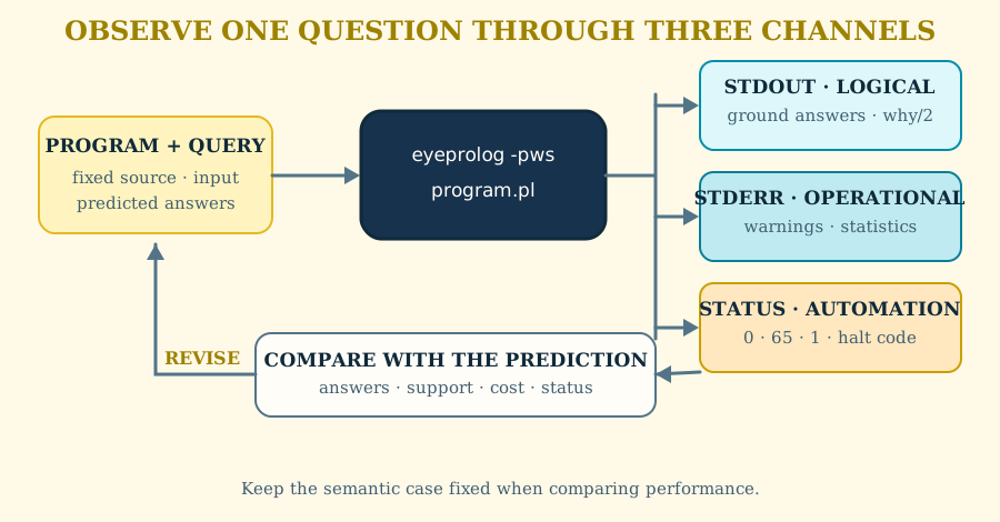
eyeprolog
eyeprolog [options] [file-or-url.pl|- ...]
Interactive queries
Run eyeprolog without arguments to enter the interactive top level. Queries
may span lines and end with a full stop, as in Scryer Prolog:
?- use_module(library(lists)).
   true.
?- member(X, [prolog, logic]).
   X = prolog
;  X = logic.
?- halt.
When another answer exists in an interactive terminal, press ;, Space, or
n to ask for it immediately; no Return is needed. Return or . stops
enumeration, a enumerates all remaining answers, and f advances to the
next five-answer boundary (5, 10, 15, … displayed leaf answers), regardless
of how many answers were stepped through individually beforehand. h displays
the answer-control help. Enumeration of goal continuations is demand-driven:
after an answer is found, the top level does not execute a later program branch
or side effect merely to discover whether the current answer is the last one.
The solver’s uniform choicepoint protocol uses explicit clause and control
frames, permits a one-answer buffer only for effect-free host relations, and
requires stateful or meta-control iterators to report their pending state
directly. Search that can perform an effect starts only after an answer-control
command asks to continue. Stopping enumeration closes any active
call_cleanup/2 or
setup_call_cleanup/3 protection exactly once; detecting that a choicepoint
remains does not execute that next branch. If an unresolved alternative
ultimately has no solution, asking for it may therefore finish with false.. In scripted non-TTY input, a new
query line implicitly stops the preceding answer enumeration without consuming
the new query; explicit ;, n, Space, a, or f still requests more
answers. Once the top-level reader has accepted a complete query, the following
line begins with two spaces to mark active execution; a
third space appears when its result is ready for formatting. The answer prompt
is ; with no trailing space while it waits for input; after an advance
command, one space marks active search and a second marks an answer ready for
formatting. While a query is actively computing, EyeProlog releases readline’s
terminal signal handling: Ctrl-C
therefore terminates the current EyeProlog process immediately, and on POSIX
terminals Ctrl-Z suspends it in the usual shell-managed way. This remains a
host top-level convention rather than an ISO/IEC 13211-1 language feature. A
period-terminated query with no solutions prints false.. A solution without
visible variable bindings prints true. only when it also has no pending
residual goals. Residual constraints are part of the displayed answer even when
the attributed variable was created inside a called predicate and is not a
visible query variable; the top level assigns such variables generated names
like _A. For example, if ffalse :- freeze(_, false)., the query ffalse.
displays freeze:freeze(_A, false)., and
call_residue_vars(ffalse, Vs). displays
Vs = [_A], freeze:freeze(_A, false). rather than implying that the returned
variable is unconstrained. Answer substitutions are rendered as valid Prolog
syntax under the current operator table: when a bound value would
not be a valid right operand of the displayed =/2, EyeProlog adds parentheses,
for example T = (a = b). rather than the invalid T = a = b.. When an answer
ends in a graphic token, the top level inserts layout before its terminating
full stop so the two tokens cannot merge; for example ?- X = .* . displays
X = .* ., not X = .*.. Use [file]., ['file.pl']., or
consult(file). to consult local source; reconsult(file). is accepted as a
compatibility alias. Use halt. or halt(Status). to leave the top level.
For an extensionless designation such as [file]. or consult(file)., the
top level tries file.pl before the unsuffixed file. Both the shorthand and
consult/1 have modern reconsult semantics: consulting the same resolved file
again replaces its previous source, so clauses removed from the file do not
remain active. The traditional [user]. form consults source directly from the
top-level input until end_of_file. or input EOF, rather than resolving user
as a filesystem path; consult(user). and reconsult(user). use the same
interactive source.
When read/1-2 or read_term/2-3 actually reaches interactive
user_input, the top level requests the next full-stop-terminated Prolog term
with a |: input prompt instead of treating the terminal stream as already
exhausted. The request is made at execution time, so multiple reads in one goal
and reads reached through user predicates work independently. For example:
?- read(X), read(Y).
|: hello.
|: world.
   X = hello, Y = world.
Typing Ctrl-D at an empty |: prompt makes that Prolog read return
end_of_file; it does not close the surrounding EyeProlog top-level loop, so a
new ?- query can still be entered afterwards. The top-level prompts and this
terminal EOF convention are host-interface behavior rather than part of
ISO/IEC 13211-1; terms supplied to the reads are parsed by the same ISO
term-input machinery as read/1-2 and read_term/2-3 on other text streams.
Up and Down recall queries from the current session. Explicit eyeprolog -h
displays command-line help.
Selecting goals
A Prolog source file states facts, rules, and ISO directives; the command line
selects what to solve. Supply -g or --goal followed by a callable Prolog goal:
eyeprolog --goal 'ancestor(ada, Who)' examples/ancestor.pl
Repeat -g or --goal to request several result relations in one run. EyeProlog prints
their ground answers in the order the goals were supplied.
Use --quiet for command-style goals: Prolog output such as write/1 remains
visible, while the resolved answer terms are suppressed.
A program can also carry its own question. Write it as an ISO query, or as that same query in a comment:
?- ancestor(ada, Who).      % run by this and any other ISO processor
%% ?- ancestor(ada, Who).   % run by this one, invisible to the rest
When no -g or --goal option is present, the CLI runs the queries it finds
in the input sources, in source order; an explicit goal option overrides them.
Both spellings are extensions, in the precise sense of 7.7.3: “the method by
which a user delivers a goal to the Prolog processor shall be implementation
defined”. A Prolog text itself (6.2.1) holds only :- directive-terms and
clause-terms, and the standard’s own query (3.143) is interactive top-level
input it does not require a processor to have. What the two spellings differ
in is who else runs them. A ?- term is the notation nearly every Prolog
uses for a goal, and the one eyeron’s documented subset defines, so a program
written that way runs in both engines; --iso-strict does not accept it. A
%% ?- comment is invisible to every other processor, which keeps a file
portable to the external Prologs the conformance harness runs it through. The
standard’s own way to put a goal in a text is :- initialization(Goal).
(7.4.2.6), which works here too. External goals remain preferable when a
script, shell history, or API call should make the observed question
explicit.
| Option | Meaning |
|---|---|
-h, --help |
Show usage |
-p, --proof |
Print why/2 explanations |
--proof-detail abstract|expanded |
Select library abstraction for proof output; implies --proof |
--check-proof File |
Check a saved proof document against the input program without proof search, writing the result as condition/4, failure/3, obligation/3 and verdict/1 facts; - reads the proof from stdin |
-q, --quads |
Run embedded quad tests and fail if any do not hold |
--quiet |
Suppress resolved answer terms while preserving Prolog output and diagnostics |
--iso-strict |
Restrict parsing and execution to ISO/IEC 13211-1:1995 + Corrigenda 1–3; reject EyeProlog language extensions (including table and :+) and disable bundled-library autoloading |
--portable |
Enforce the conservative EyeProlog/Trealla/Scryer interoperability profile |
--no-autoload |
Disable bundled-library predicate autoloading |
-s, --stats |
Print final solver and memory statistics to stderr after execution |
-v, --version |
Print the package version |
-w, --warnings |
Print non-fatal portability warnings |
-g, --goal Goal |
Solve a callable goal; may be repeated; overrides queries in the source |
-- |
Treat following arguments as inputs |
Short flags may be combined, so -pqw is equivalent to -p -q -w.
--iso-strict cannot be combined with --quads, because quads and their
predefined infix (?-)/2 form are an EyeProlog testing extension. Strict mode
retains the Part 1 prefix (?-)/1 operator and treats -->/2 as ordinary Part
1 operator syntax; it does not perform Part 3 grammar-rule expansion or expose
phrase/2-3. Part 2 module directives and EyeProlog libraries are rejected,
the implementation-specific occurs_check flag is absent, and the normal-profile
table declaration is unavailable. Normal mode continues to support Parts
2–3 and EyeProlog extensions, plus generated autoloading across the bundled
src/lib/ library exports documented above.
Inputs may be local files, HTTP(S) URLs, or one - for stdin. The bare command
eyeprolog starts the normal REPL; eyeprolog --iso-strict starts the strict
core REPL. When options are present but no input is named, stdin is normally
used, but the strict-mode-only invocation is reserved for the REPL, so write
eyeprolog --iso-strict - explicitly when strict source should come from
stdin. Multiple sources are parsed as one program, so facts, rules, and
directives can be separated across files. A relative include/1 inside a local
file resolves from that file’s directory.
For example:
eyeprolog --iso-strict --goal 'p(X)' program.pl
eyeprolog --iso-strict
printf 'p(a).\n' | eyeprolog --iso-strict --goal 'p(X)' -
A reproducible run
Work in a fixed sequence:
- predict the ground answers before running the program;
- run without observation flags and compare stdout with that prediction;
- add
--proofwhen the support for an answer is the question; save the output and use--check-proofwhen the derivation itself must cross a process or review boundary; - add
--warningswhen portability or negative dependencies are the question; use--portablewhen non-profile dependencies must fail CI; - add
--statsonly when comparing two executions of the same semantic case.
For example:
eyeprolog --goal 'ancestor(X, Y)' examples/ancestor.pl
eyeprolog --proof --goal 'type(X, Y)' examples/socrates.pl
eyeprolog --proof examples/socrates.pl > socrates.why.pl
eyeprolog --check-proof socrates.why.pl examples/socrates.pl
eyeprolog --warnings --goal 'answer(X)' test/conformance/warnings/negation/unstratified_mutual.pl
eyeprolog --portable --goal 'sudoku9(S)' examples/clpz-sudoku-9x9.pl
eyeprolog --stats --goal 'path(a, X)' examples/path-discovery.pl > answers.pl 2> run.stats
Normal answers and why/2 terms go to stdout, which makes them suitable for a
golden file or another EyeProlog input. Warnings and statistics go to stderr so
they do not corrupt that logical stream. A successful run normally exits with
status zero; loading, syntax, option, and other uncaught errors use status 1. halt/0-1 can deliberately choose the
process status from inside a program.
Embedded quad tests
A quad places a query directly before a description of its expected top-level answer. The answer is ordinary Prolog syntax rather than quoted text or a comment, so a small test reads like the interaction it checks:
color(red).
color(green).

colors ?- color(X).
   X = red
;  X = green.

?- color(blue).
   false.
Run all quads in a file with eyeprolog --quads file.pl or eyeprolog -q
file.pl. A label such as colors is optional. A label is not a separate
mini-language: it is the ordinary first argument of (?-)/2, and therefore may
be any Prolog term admitted there by the normal term grammar. Quad execution
requires that argument to be ground; a non-ground label is reported as a quad
failure rather than aborting source parsing. Loading the file normally only
records its quads; it does not execute them or add their queries and answers as
program clauses. A quad run prints a summary and exits with status 1 when any
description fails. If no description fails but a bounded search cannot decide
an exact answer sequence, the case is reported separately as UNDECIDED and
the CLI exits with status 2. Quad mode imports library(prologue) as a
compatibility prelude because the ISO Prolog working-example files use those
predicates as system predicates without an explicit module directive.
Unless the source explicitly selects another unknown flag, quad execution
uses unknown=error, so an undefined predicate is reported rather than being
accepted as a negative answer.
Answer descriptions support ordered answers separated by ;, acceptable
alternatives separated by |, true, false, standard error descriptions,
and the unexpected annotation for an answer that must not occur (inattendue
is its synonym). In an ordered answer sequence, unexpected is a negative
assertion about the answer at that position: once the next observed answer does
not match the annotated leaf, that description succeeds and does not require the
query to have no further answers. Variables named in the query keep their
identity inside answer descriptions; variables introduced only by a description
are fresh. For example,
a query throw(g(X)) is described by throw(g(_X)), while
throw(g(X)), unexpected verifies that ISO throw/1 did not retain the query
variable in the renamed exception term. ... and ad_infinitum accept further answers. The maybe annotation describes
a successful answer that still has at least one pending residual constraint. It
does not stand for an arbitrary answer and it does not weaken substitution
matching: X = a, maybe still requires the X = a substitution. Conversely, a
successful answer description without maybe requires that no residual
constraint remain. For example, a pending dif/2 constraint can be checked as:
?- dif(X,Y), X = a.
   true, unexpected.
   X = a, unexpected.
   X = a, maybe.
   maybe, unexpected.
ISO arithmetic examples sometimes describe a floating result only as
“approximately equal” to a written decimal. Quad answer descriptions preserve
the precision of that spelling with ~~: the right-hand side is a decimal atom,
so trailing zeroes remain significant. V ~~ '14.2000' accepts a float in
the closed decimal interval 14.19995 through 14.20005; it does not accept an
integer term, even when that integer has the same mathematical value. Exponent
notation uses the last written mantissa digit in the same way, so '1.42000e1'
denotes the same interval. For example:
?- V is 0+(3.2+11).
   V ~~ '14.2000'.
~~ is an EyeProlog normal-profile operator at priority 700 with specifier
xfx, matching the priority/specifier of ISO comparison operators such as =;
there is no built-in ~~/2 predicate. Quad answer descriptions interpret the
operator specially as approximate float matching.
An approximation is accepted as well-formed only when its exact decimal interval contains at least three distinct, strictly ascending finite EyeProlog floats: the minimum representable float in the interval, the float denoted by the written midpoint, and the maximum representable float in the interval. This prevents a decimal spelling from claiming precision finer than the implementation can represent, including decimal spellings whose apparent precision collapses to the same implementation float, and rejects ranges that would require non-finite continuation values. Endpoint selection is directed inward, so a binary rounding of a decimal bound cannot admit a float that lies mathematically outside the closed decimal interval.
A numeric right-hand side such as V ~~ 14.2000 is deliberately rejected
because parsing it as a float would discard the written decimal precision that
the check is intended to retain.
EyeProlog treats native variable constraints, attributed-variable residue, and
delayed goals as pending residue for this purpose. Multiple
indented descriptions after one query are independent checks: each re-runs the
query, each is counted in the quads: summary, and a failing description does
not suppress later descriptions for that query. inputs/1 supplies and checks
exactly the characters consumed by the query. peeks/1 may add one character
that is available for look-ahead but must remain unconsumed. The runner puts an
invalid-character sentinel immediately after the declared input boundary, so a
reader cannot accidentally use an artificial end-of-file to decide that a full
stop terminates the term. For example:
?- read(X).
   inputs("1."), X = 1, unexpected.
   inputs("1."), peeks(" "), X = 1.
   inputs("1. "), peeks(" "), X = 1, unexpected.
outputs/1 checks characters emitted while reaching the described answer or
error, including output produced before a later exception. Its argument may be
an exact character list/string or a DCG body: terminal sequences,
conjunction/disjunction, .../ad_infinitum sequence wildcards, and
user-defined DCG nonterminals are matched against the captured characters.
Appending | other_answer_sequence accepts any permutation of the preceding
complete answer sequence. Substitutions, residual constraints, per-answer output,
and duplicate counts must still match; missing or extra answers are failures.
A final failure or exception stays at the end. Overlapping wildcard or approximate
answer descriptions are matched one-to-one rather than greedily. Search-budget
exhaustion remains undecided. Prefix (...), negative (unexpected), STO, and
input/wait annotations are not supported in a permuted sequence.
For setof(1, (Y=2 ; Y=1), L), the description
Y=2, L=[1] ; Y=1, L=[1] | other_answer_sequence accepts either group order.
STO, loops, and undecided quad results
Following Trealla’s quad convention, sto declares that a query is subject to
occurs-check. EyeProlog checks this conservatively rather than attempting a
complete STO/NSTO decision procedure. During the query’s ordinary execution,
the finite-tree unifier records a concrete occurs-check event as positive STO
evidence; the query is not run a second time merely to probe STO-ness. A finite
execution that completes naturally without such an event disproves sto, while
a search or resource boundary leaves the declaration conservatively unchecked.
The answer portion of an sto-annotated leaf remains implementation-dependent
and is therefore not compared.
For example, the cyclic binding in the first query provides positive STO evidence, whereas the second query is finite and cannot be STO:
?- X = s(X).
   X = ..., unexpected.
   false, unexpected.
   sto, false
|  sto, true.

?- true.
   sto.                  % fails: no STO evidence
When a quad declares STO and the execution observes an occurs-check event, an
unannotated unexpected leaf does not reject the implementation-dependent
finite-tree outcome. This is partial STO detection only: EyeProlog makes a
definite statement where execution provides definite evidence and otherwise
does not guess.
loops is kept distinct from merely exhausting the quad runner’s resources.
EyeProlog accepts structural nontermination evidence such as an active-variant
recursion cycle, with the loop depth/inference bounds as a bounded fallback. A
structural cycle is also strong enough to refute a finite false description;
it is not reported as undecided merely because the same query was checked by a
different answer description:
inf :- inf, inf.

?- inf.
   loops.
Ordinary answer descriptions also have a finite inference budget (100000 by
default). Exhausting that budget does not establish loops and does not
turn an unfinished search into false; instead the description is reported as
UNDECIDED, for example:
quads: UNDECIDED expensive_case, program.pl:12
   undecided: inference limit reached.
Thus quad execution has three useful outcomes: passed, failed, and undecided.
When there are no failures but at least one undecided description, the CLI exits
with status 2. The JavaScript API may override the ordinary search budget with
quadMaxInferences; loopMaxDepth and loopMaxInferences control the explicit
loops probe.
The JavaScript API exposes the same operation without process I/O:
import { Program, runQuads } from 'eyeprolog';

const program = Program.parse(source);
const report = runQuads(program);
console.log(report.passed, report.failed, report.undecided, report.stdout);
The syntax follows the “queries using answer descriptions” convention used by
Trealla and the ISO Prolog working examples. Because answer descriptions are
layout-sensitive, indent every description while keeping ordinary clause heads
and the next quad query at the left margin. A quad label may contain any number
of comma-separated metadata fields, including across layout before ?-; for
example 9, "case", passes ?- Goal. is one labelled query. Quad recognition
is structural after ordinary term parsing: functional, mixed, quoted-functor,
and parenthesized spellings of the same ?-/1 or ?-/2 term are semantically
equivalent. For example ?-(Label, Query). and (?-(Label, Query))., followed
by the same indented answer descriptions, create the same labelled quad as
Label ?- Query..
Statistics are comparative evidence, not a score in isolation. Preserve the program, input, runtime version, selected query, answers, and counters together. An optimization is acceptable only when the intended answers remain unchanged and the chosen resource measure improves on the relevant scale case.
The corpus as executable documentation
The files under examples/ pair readable programs with checked output under examples/output/. The conformance cases under test/conformance/ focus on language behavior, including success, failure, errors, warnings, and file loading. Use an example to learn a modeling pattern and a conformance case to settle an exact processor question. Run npm test to execute the complete correctness corpus.
Checkpoint. Run one example with --proof --stats. Identify which bytes
belong to the reusable logical result, which describe this execution, and which
process status an automated caller observes. Then change one fact and predict
all three channels before rerunning it.
41. Study paths, review, and further examples
For a first week, run socrates.pl and ancestor.pl, rewrite them from memory,
inspect their proofs, learn member/2, append/3, and select/3, solve one
finite puzzle, and add one explicit integrity query.
Course-length schedules
These schedules name a spine rather than a reading quota. Every meeting should include prediction, execution, one changed input, and a short explanation.
| Meeting | Six-meeting introduction | Ten-meeting course | Fourteen-meeting course |
|---|---|---|---|
| 1 | Chapters 1–2; Socrates and family facts | Chapters 1–2; Laboratory 1 begins | Chapters 1–2; predicates, terms, and unification |
| 2 | Chapters 3–5; recursion and lists | Chapters 3–5; Laboratories 1–2 | Chapters 3–4; rules, semantics, and recursion |
| 3 | Chapters 6–10; one finite puzzle | Chapters 6–8; finite generation and absence | Chapters 5–6; lists and arithmetic |
| 4 | Chapters 11–14 and 17–20; proof, integrity, construction | Chapters 9–12; contexts, models, proofs, and integrity checks | Chapters 7–8; negation and aggregation |
| 5 | Choose Chapters 21–25 or 26–30 | Chapters 13–16; performance and boundaries | Chapters 9–10; structured data and finite models |
| 6 | Chapters 31–33; release matrix and reflection | Chapters 17–20; construction and improvement | Chapters 11–12; answers, proofs, and integrity |
| 7 | — | Chapters 21–25; one advanced case | Chapters 13–14; termination and knowledge engineering |
| 8 | — | Choose Chapters 26–30 | Choose Chapters 15–16 or an alternate domain route |
| 9 | — | Chapters 31–32; test and debug | Chapters 17–20; construction, correctness, improvement |
| 10 | — | Chapter 33; project review | Chapters 21–25; advanced relational design |
| 11 | — | — | Chapters 26–27; witnesses and induction |
| 12 | — | — | Chapters 28–30; representation, experiment, limits |
| 13 | — | — | Chapters 31–33; test, debug, patterns |
| 14 | — | — | Laboratory demonstrations and rubric review |
For a classroom, use checkpoints as exit questions and laboratories as multi-meeting projects. A six-meeting introduction should prefer one small, finished theory over hurried coverage of every feature.
Domain routes
Modelers should study access-control-policy.pl,
clinical-trial-screening.pl, gdpr-compliance.pl, and
trust-flow-provenance-threshold.pl. Identify facts, derived concepts,
decisions, closed-world assumptions, and proof premises.
Algorithm students should study graph-reachability.pl,
dijkstra-risk-path.pl, stable-marriage.pl, sat-solver-dpll.pl, and
type-inference.pl. For each, identify the finite domain, branching relation,
pruning goals, witness, and termination argument.
Mathematics students should read Chapters 3, 19, and 26–30 together, then study
peano-calculus.pl, fundamental-theorem-arithmetic.pl,
stirling-bell-numbers.pl, d3-group.pl, and
matrix-noncommutativity.pl. For each program, distinguish definition from
theorem, computation from justification, finite evidence from universal proof,
and syntactic equality from the domain’s mathematical equality.
Review questions
Review questions:
- What distinguishes an atom constant from an atomic formula?
- Why can one append relation construct lists and split them?
- When does goal order affect performance but not declarative meaning?
- Why should variables usually be bound before
\+/1? - What does explicit tabling solve, and when should a predicate remain depth-first?
- Why is proof output useful when the answer is already known?
- When should a host query an
invalid/1relation before domain decisions? - Why should external data conversion remain outside the reasoning core?
- In what sense is a ground query answer an existential witness?
- Why are partial correctness, completeness, and termination three different claims?
- When can exhaustive computation constitute a proof, and when is it only evidence?
- Which parts of an answer’s trust come from its proof, and which remain outside the formal theory?
Further examples
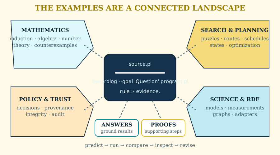
The examples directory is the book’s executable companion. The
top-level directory contains 236 self-contained runnable programs. Every
source program has an exact answer file under
examples/output, and 236 programs have a checked
explanation under examples/proof together with the result of that
check under examples/check. A check result is itself ordinary Prolog
— condition/4 for each of the five conditions, failure/3 for anything that
did not hold, one obligation/3 naming each conclusion the check rests on
rather than establishes, counts including composed/1 for conclusions carried
by the goals they wrap, and verdict/1 — so the same reasoning that produced an answer
can be turned on the question of whether that answer was checked. Every one of those explanations is re-checked by npm test, which
re-performs each recorded inference against its source clause and recomputes
each primitive the document asserts. The thematic lists link every top-level program and open the program
itself rather than merely naming it.
examples/book/ mirrors the inline EyeProlog displays chapter by chapter. Those files are checked for syntax, and displays containing queries are executed, but some teaching fragments deliberately depend on neighboring facts or helpers. Use the top-level examples when you want a self-contained program with a golden answer; use examples/book/ when you want the exact display being discussed on a page.
Every example is packaged as an answer, a reason, and a check, because those are three different claims and only the first is what a program usually returns:
- source: the facts, rules, comments, and declared queries in the top-level examples directory;
- answer: the exact normal output, in its
examples/output/counterpart. It says what follows, and on its own it asks to be taken on trust; - reason: the exact
--proofoutput, in the correspondingexamples/proof/file. It says why it follows, asstep/4facts naming the clause each conclusion used and what it rested on. A reader can now follow the derivation instead of trusting it — but following it is their work, and a long derivation is not something a person checks by reading; - check: the exact
--check-proofoutput, inexamples/check/. It says whether that reason holds, decided mechanically and not by the engine that produced the answer. A proof can be internally flawless and still record a value that is simply false, which is why the third view is worth more than the second: it is the one that can come back and say no.
A check document is itself ordinary Prolog, so the last view is not a report to
read but a result to reason over: condition/4 for each of the five
conditions, failure/3 for anything that did not hold, and one obligation/3
naming each conclusion the check rests on rather than establishes.
Run one program directly:
node bin/eyeprolog.js examples/ancestor.pl
node bin/eyeprolog.js --proof examples/ancestor.pl
Then compare the result with its linked golden file. A productive reading sequence is:
- read the query declarations and predict their ground answers;
- identify facts, base clauses, recursive clauses, and mode-sensitive built-ins;
- state one intended mode and its finiteness argument;
- run the program and compare with the answer golden;
- inspect the proof, when supplied, and mark which source clauses support the conclusion;
- change one fact or bound and predict the changed answer before rerunning.
Standard Prolog profile
These examples compose ISO facilities that isolated conformance cases test one mode at a time.
| Program | Standard facility | Answer · reason · check |
|---|---|---|
| CLP(B) Boolean circuit | A NOT/AND/OR XOR circuit is enumerated with labeling/1, then taut/2 verifies equivalence to the XOR (#) specification. |
answer · reason · check |
| CLP(B) cardinality | A two-of-four review quorum combines card/2, implication, exclusive-or, labeling, and model counting. |
answer · reason · check |
| CLP(B) feature model | Deployment-feature dependencies are expressed as Boolean constraints, enumerated with labeling/1, and counted directly with sat_count/2. |
answer · reason · check |
| CLP(B) weighted planning | A bounded release plan uses implications and cardinality constraints, then weighted_maximum/3 selects the highest-value admissible feature set. |
answer · reason · check |
| CLP(Z) factorial | Declarative predecessor and product constraints propagate a factorial without mode-sensitive is/2. |
answer · reason · check |
| CLP(Z) global constraints | Compatibility tables, lexicographic and serialized schedules, global cardinality with costs, circuits, value counting, and integer comparison. | answer · reason · check |
| CLP(Z) N-queens | A checked eight-queens witness using finite domains, delayed diagonal constraints, all_distinct/1, and first-fail labeling, plus a four-queens multi-solution search. |
answer · reason · check |
| CLP(Z) resource allocation | Resource assignment using element/3, sum/3, scalar_product/4, reification, labeling options, and domain reflection. |
answer · reason · check |
| CLP(Z) Sudoku 9×9 | The AI Escargot 9×9 model with finite domains, 27 all-distinct constraints, and first-fail labeling, genuinely searched from its clues as the default example goal. | answer · reason · check |
| Combinatorics Findall Sort | Eyelet-inspired combinations example using findall/3 and ISO sort/2. |
answer · reason · check |
| Floating Point | Floating-point arithmetic and comparisons. | answer · reason · check |
| Atomic conversion | Atom splitting, character atoms, Unicode codes, and numeric parsing. | answer · reason · check |
| Control and errors | call/1, once/1, cut, if-then-else, throw/1, and catch/3. |
answer · reason · check |
| DCG command parser | A Part 3 grammar parses token lists into application terms, generates tokens, preserves a remainder, and rejects malformed input. | answer · reason · check |
| DCG expression language | A precedence-aware bidirectional grammar builds arithmetic ASTs, evaluates variable expressions, regenerates minimally parenthesized tokens, round-trips syntax, and preserves a remainder. | answer · reason · check |
| Dynamic database | Initialization and ordered updates to a declared dynamic procedure. | answer · reason · check |
| Grouped solutions | findall/3, bagof/3, setof/3, existential qualification, and clause/2. |
answer · reason · check |
| Integer arithmetic | Integer quotient/remainder choices plus bit operations. | answer · reason · check |
| ISO extension pipeline audit | A bounded pipeline audit composing every library(iso_ext) relation: nested counting, universal validation, successor generation, difference-list collection, and schema comparison modulo variable names. |
answer · reason · check |
| ISO extensions | Common control, collection, integer, and term-variant extensions from library(iso_ext). |
answer · reason · check |
| Operators | Custom syntax, standard term order, and operator-table inspection. | answer · reason · check |
| Portable library overlap | Shared Scryer/Trealla interfaces for CLP(B), ordered sets, graphs, reification, delayed goals, generated names, character conversion, matrix transposition, and explicit table syntax. | answer · reason · check |
| Reflective terms | Term shape, construction, copying, variables, identity, and standard order. | answer · reason · check |
| Term I/O | Text-stream lifecycle, canonical writing, reading, metadata, and end state. | answer · reason · check |
| Term Tools | Term-tool builtins for inspecting, constructing, rendering, and validating structured terms. | answer · reason · check |
| Aliases and namespaces | One native spelling per built-in, with vocabulary-style names layered above it. | answer · reason · check |
| Attributed variables | Scryer-style attributed variables over the annotated-variable runtime. | answer · reason · check |
| dif constraints | Delayed disequality with dif/2, which waits rather than guessing. | answer · reason · check |
| Reified conditionals | A condition carried as a value, so a test can be reasoned about rather than only run. | answer · reason · check |
| Bulk stream write | Character-by-character writes to a non-console text stream. | answer · reason · check |
| JSON | JSON parsing and generation in the shared Scryer/Trealla representation. | answer · reason · check |
| HTTP client | HTTP/HTTPS requests from the bundled client library. | answer · reason · check |
Read these beside Part VIII. Then use the ISO conformance cases when a program depends on the exact failure or error behavior of a particular mode.
First encounters
These programs isolate one idea at a time. Read them before the larger case studies.
| Program | What to notice | Answer · reason · check |
|---|---|---|
| Age | Arithmetic comparison acts as a filter after a fact supplies the age. | answer · reason · check |
| Ancestor | The canonical base-plus-recursive definition computes a transitive family relation. | answer · reason · check |
| Animal | Several clauses form a small classification theory with inspectable reasons. | answer · reason · check |
| Annotation | Terms attach descriptive data while the logical relation remains ordinary. | answer · reason · check |
| Backward | A tiny derived fact justified by a numeric comparison in an ordinary Horn rule. | answer · reason · check |
| Cat Koko | Named Skolem-style witnesses standing in for the existential witnesses of the original N3 example. | answer · reason · check |
| Derived rule | A conclusion depends on another derived predicate rather than directly on a source fact. | answer · reason · check |
| Dog | A compact inheritance chain shows how intermediate concepts appear in a proof. | answer · reason · check |
| Existential rule | Structured Herbrand terms carry explicit generated witnesses. | answer · reason · check |
| Good cobbler | Multiple premises combine into a conclusion without hidden mutation or control state. | answer · reason · check |
| Herbrand Semantics | Herbrand terms denote themselves: distinct names and constructor applications remain distinct without extra unique-name or free-constructor axioms. | answer · reason · check |
| Herbrand witnesses | Functional witness terms make existential structure and syntactic identity visible in both answers and derivations. | answer · reason · check |
| Reusable built-ins | Arithmetic, strings, lists, and term inspection compose through ordinary variables. | answer · reason · check |
| Skolem Functions | Skolem functional terms in rule heads. | answer · reason · check |
| SNAF | Negation as failure establishes that Alice does not hate Bob before deriving that she hates Nobody. | answer · reason · check |
| Socrates | A fact and one rule turn the classical syllogism into a ground derivation. | answer · reason · check |
| UUID | uuid/3 reproducibly creates one version 4 UUID atom from explicit random state; the example validates its canonical shape. |
answer · reason · check |
| Witch | Burn the witch, adapted from Eyeling’s examples/witch.n3. | answer · reason · check |
Suggested path: Socrates → Age → Ancestor → Derived rule → Reusable built-ins. At each step, say aloud what one ground instance of every predicate means.
Recursion, lists, and graph closure
These examples make termination arguments visible. Compare structural descent, visited-state search, and fixed-point tabling rather than treating all recursion as one technique.
| Program | What to notice | Answer · reason · check |
|---|---|---|
| Chart parser | A finite chart represents shared parsing subproblems and recursive grammatical structure. | answer · reason · check |
| Cyclic path | A deliberately cyclic graph exposes repeated calls and the need for disciplined recursion. | answer · reason · check |
| Deep taxonomy: 10 | A small generated hierarchy is readable by hand and establishes the benchmark shape. | answer · reason · check |
| Deep Taxonomy 100 | A 100-step taxonomy chain that exercises deep recursive closure and side-label derivation. | answer · reason · check |
| Deep taxonomy: 1,000 | The same logical theory tests indexing and recursive closure at a realistic depth. | answer · reason · check |
| Deep Taxonomy 10000 | A 10,000-step taxonomy chain used as a large-depth ordinary-recursion and closure stress test. | answer · reason · check |
| Deep taxonomy: 100,000 | A stress case separates semantic simplicity from implementation scale. | answer · reason · check |
| Family cousins | Several relational joins derive kinship beyond a simple transitive closure. | answer · reason · check |
| Graph reachability | A visited list bounds cyclic traversal and makes explicit negative test cases finite. | answer · reason · check |
| Graph | Productive right-recursive transitive closure over a directed map, contrasted with an under-generating left-recursive formulation. | answer · reason · check |
| List collection | findall/3, list construction, and aggregation turn a solution stream into data. |
answer · reason · check |
| Path discovery | Witness paths, not only endpoint pairs, are constructed during a larger graph search. | answer · reason · check |
| Service Impact | Practical cyclic recursion: incident impact analysis for a service dependency graph. | answer · reason · check |
| Naive reverse benchmark | Quintus’s 1984 naive-reverse benchmark, kept as a readable recursion. | answer · reason · check |
Read the three taxonomy programs as one experiment: the mathematical relation does not change as the data scale changes. Any difference in runtime belongs to control, indexing, memory, and table management.
Finite search, puzzles, and optimization
The central question for every program in this group is: what exactly is the finite search space, and which constraint removes which branches?
| Program | Search design | Answer · reason · check |
|---|---|---|
| Dijkstra Findall Sort | Eyelet-inspired Dijkstra example using findall/3 and ISO sort/2. |
answer · reason · check |
| Dijkstra | Weighted path enumeration adapted from Eyeling dijkstra.n3. | answer · reason · check |
| DONALD + GERALD = ROBERT | All ten decimal digits are assigned to ten distinct letters. Right-to-left carry propagation cuts a naive 10! search space to one solution. | answer · reason · check |
| Enigma1225 | New Scientist Enigma 1225, retaining the best board in one pass with aggregate_max/5. |
answer · reason · check |
| Eulerian path | The state tracks remaining edges rather than merely visited vertices. | answer · reason · check |
| Four-color map | A finite color assignment is filtered by adjacency constraints. | answer · reason · check |
| Hamiltonian path | A witness must visit every vertex exactly once; path construction and global coverage meet. | answer · reason · check |
| Job-shop scheduling | Resource and precedence constraints interact in a larger finite schedule space. | answer · reason · check |
| Knapsack optimization | Candidate subsets become feasible solutions, then aggregation selects a best value. | answer · reason · check |
| Map Four Color Search | Four-colour search for the European Union neighbour graph. | answer · reason · check |
| Markov Logic Network | Markov Logic Network style scoring over a tiny finite domain. | answer · reason · check |
| Matrix Chain Order | Matrix-chain multiplication order by explicitly tabled interval dynamic programming. | answer · reason · check |
| Register allocation | Interference constraints turn compiler allocation into graph coloring. | answer · reason · check |
| SEND + MORE = MONEY | Digit assignments are generated under distinctness, leading-zero, and column constraints. | answer · reason · check |
| Stable marriage | Preference data, matching generation, and the absence of blocking pairs define stability. | answer · reason · check |
| Weighted interval scheduling | Compatibility constraints and an ordered objective select a maximum-value schedule. | answer · reason · check |
| Zebra puzzle | House records, adjacency relations, and clue constraints jointly determine the famous solution. | answer · reason · check |
| Knight’s tour (Warnsdorff) | A heuristic that moves to the most constrained square first. | answer · reason · check |
A useful comparative exercise is to draw the first three levels of the search tree for N-Queens, SEND + MORE = MONEY, DONALD + GERALD = ROBERT, and Knapsack. Mark whether each branching decision chooses a permutation element, assigns a digit, derives a carry-constrained digit, or includes an item. The syntax is similar; the combinatorial objects and pruning strength are different.
Planning and state transition
Planning programs represent a world state as a term, define legal transitions, and search for a sequence whose final state satisfies a goal.
| Program | State-space idea | Answer · reason · check |
|---|---|---|
| Allen Interval Calculus | Allen interval relations over integer time offsets, with interval records kept as scoped data. | answer · reason · check |
| Blocks world | Symbolic actions transform a compact arrangement of blocks. | answer · reason · check |
| Critical-path schedule | Dependency closure and duration arithmetic derive project timing. | answer · reason · check |
| Dijkstra Risk Path | Risk-adjusted route selection that combines delivery cost, accumulated risk, path length, and a trust gate. | answer · reason · check |
| Dining Philosophers | Chandy-Misra dining philosophers trace adapted from Eyeling dining-philosophers.n3. | answer · reason · check |
| Drone corridor planner | Route feasibility combines graph structure with domain restrictions. | answer · reason · check |
| GPS | Route planning over scoped map data, accumulating actions, duration, cost, belief, and comfort. | answer · reason · check |
| Gray Code Counter | Gray-code counter adapted from Eyeling gray-code-counter.n3. | answer · reason · check |
| Hanoi | A recursive plan mirrors the inductive structure of moving a tower. | answer · reason · check |
| Lee routing | Breadth-first wave expansion reaches a destination on a grid, then reconstructs a path around rectangular obstacles using the standard list relations. | answer · reason · check |
| Microgrid dispatch | Candidate operating decisions are checked against supply, demand, and engineering limits. | answer · reason · check |
| Missionaries and cannibals | Numeric state constraints must hold on both banks after every crossing. | answer · reason · check |
| Monkey and bananas | Actions change location, support, and possession facts until the goal becomes true. | answer · reason · check |
| Route planning | Weighted edges construct candidate routes and expose the chosen path as a witness. | answer · reason · check |
| Wolf, goat, and cabbage | Safety invariants reject river-bank states before they enter a valid plan. | answer · reason · check |
Compare the witness shape: Hanoi returns an inductively constructed move list; route planning returns a graph path; Lee routing reconstructs a path from breadth-first wave layers; Blocks world and the river puzzles expose a sequence of whole states. Representation determines which plan properties are easy to check.
Mathematics as relations
These examples accompany Part VI. They range from executable definitions to finite counterexample searches. Do not call every computed result a theorem: state which domain was exhausted and which general property was proved only by the clauses.
| Program | Mathematical content | Answer · reason · check |
|---|---|---|
| Ackermann | Ackermann-style fast-growing recursion benchmark adapted from Eyeling ackermann.n3. |
answer · reason · check |
| Binomial Vandermonde | Two finite sums compute the sides of Vandermonde’s identity. | answer · reason · check |
| Catalan convolution | A classic convolution identity is evaluated over a bounded range. | answer · reason · check |
| Collatz 1000 | Collatz conjecture suite translated from Eyeling’s examples/collatz-1000.n3. | answer · reason · check |
| Complex | Complex numbers, adapted from Eyeling complex.n3. | answer · reason · check |
| Composition Of Injective Functions Is Injective | Composition of injective functions is injective, adapted from Eyeling’s examples/composition-of-injective-functions-is-injective.n3. | answer · reason · check |
| Continued Fraction Sqrt2 | Convergents of sqrt(2) by explicitly tabled recurrence. | answer · reason · check |
| D3 group | A finite Cayley table, inverses, and subgroup closure make group laws executable. | answer · reason · check |
| Diamond Property | Diamond property, adapted from Eyelet’s input/diamond-property.pl. | answer · reason · check |
| Easter Computus | Gregorian Easter computus adapted from Eyeling’s easter.n3. | answer · reason · check |
| Equivalence Classes Overlap Implies Same Class | Equivalence-class overlap example adapted from Eyeling. | answer · reason · check |
| Fast exponentiation | Algebraic decomposition by parity changes a linear recurrence into logarithmic-depth recursion. | answer · reason · check |
| Fibonacci | A recurrence becomes an executable relation with a visibly decreasing argument. | answer · reason · check |
| Fundamental theorem of arithmetic | Two factorization strategies construct normalized prime-factor witnesses and check reconstruction. | answer · reason · check |
| Goldbach | Bounded search checks Goldbach decompositions for powers of two using the portable Prolog primality relation. | answer · reason · check |
| Greatest lower bound uniqueness | Order-theoretic definitions support a uniqueness argument. | answer · reason · check |
| Group inverse uniqueness | A short derivation exposes the algebraic premises needed for uniqueness. | answer · reason · check |
| Heron Theorem | Heron’s theorem: area = sqrt(s(s-a)(s-b)(s-c)). | answer · reason · check |
| Integer partitions | Recursive generation constructs unordered additive decompositions without permutation duplicates. | answer · reason · check |
| Law Of Cosines | Law of cosines: c^2 = a^2 + b^2 - 2ab cos(C). | answer · reason · check |
| Matrix noncommutativity | Two concrete products provide a counterexample to universal commutativity. | answer · reason · check |
| Modular exponentiation | Intermediate reduction preserves the residue while controlling numeric growth. | answer · reason · check |
| Newton Raphson | Newton-Raphson root finding, adapted from Eyelet input/newton-raphson.pl. | answer · reason · check |
| Peano arithmetic | Explicit natural-number terms support arithmetic relations and structural recursion. | answer · reason · check |
| Peano calculus | Addition, multiplication, and factorial follow the constructors z and s/1. |
answer · reason · check |
| Peasant | Peasant multiplication and exponentiation cases, adapted from Eyelet. | answer · reason · check |
| Pell equation | Bounded generation searches for integer witnesses to a Diophantine equation. | answer · reason · check |
| Pi | The Nilakantha series is a deterministic numeric recurrence; EyeProlog recognizes its accumulator shape and executes 10,000 terms without tabling or heap growth. | answer · reason · check |
| Prime range | Bounded integer generation and divisor tests enumerate primes over an explicit finite interval. | answer · reason · check |
| Quadratic Formula | Quadratic formula over sample equations. | answer · reason · check |
| Riemann Hypothesis | A deliberately finite audit of catalogued non-trivial zeros, illustrating the boundary between evidence and universal proof. | answer · reason · check |
| Shoelace Polygon Area | Polygon area by the shoelace formula. | answer · reason · check |
| Sieve | List filtering presents a different operational route to finite prime generation. | answer · reason · check |
| Stirling and Bell numbers | Inclusion–exclusion and recurrence count set partitions in two related ways. | answer · reason · check |
| Takeuchi | The Takeuchi function as a demanding nested-recursion benchmark. | answer · reason · check |
| Totient summatory function | Divisibility, coprimality, counting, and summation compose over finite domains. | answer · reason · check |
For a focused seminar, read Peano calculus, Fast exponentiation, D3 group, Matrix noncommutativity, and Fundamental theorem of arithmetic. They exhibit, respectively, structural induction, program improvement by algebra, finite model checking, refutation by one witness, and witness-producing number theory.
Symbolic mathematics, languages, and metaprogramming
Here terms denote syntax, formulas, expressions, or programs. The crucial discipline is to keep object language and EyeProlog metalanguage distinct.
| Program | What the terms represent | Answer · reason · check |
|---|---|---|
| SAT solver: CDCL | The example extends the SAT vocabulary toward conflicts and learned information. | answer · reason · check |
| Chart parser | Shared chart items prevent grammatical subproblems from being rediscovered independently. | answer · reason · check |
| Context Schema Audit | Schema auditing for heterogeneous context terms by decomposing members with =../2 and checking predicate arity. |
answer · reason · check |
| Derived Backward Rule | Derived backward rule example adapted from Eyeling derived-backward-rule.n3. | answer · reason · check |
| Equality saturation | Repeated rewrite closure explores equivalent symbolic forms to a fixed point. | answer · reason · check |
| Expression evaluator | Arithmetic expression trees are interpreted under an explicit environment. | answer · reason · check |
| Fast Fourier Transform | Recursive evaluation builds a shared expression tree and treats graphic operators such as + and * as data atoms. |
answer · reason · check |
| Intuitionistic Logic Kripke | Intuitionistic logic emulation with a finite Kripke model. | answer · reason · check |
| Knuth–Bendix completion | Oriented equations and critical interactions seek a more canonical rewrite system. | answer · reason · check |
| Language | A small grammar recognizes a finite relational language. | answer · reason · check |
| Linear Logic Resources | Linear logic emulation with explicit consumable resources. | answer · reason · check |
| Modal Logic Kripke | Modal logic emulation with a finite Kripke frame. | answer · reason · check |
| Partial evaluator | Known inputs specialize an expression or program while unknown parts remain symbolic. | answer · reason · check |
| Polynomial | Structured coefficients and powers support symbolic polynomial operations. | answer · reason · check |
| Proof Contrapositive | Proof by contrapositive example adapted from Eyelet input/proof-by-contrapositive.pl. | answer · reason · check |
| Quine–McCluskey | Boolean minimization with the Quine–McCluskey method, including essential implicants and deterministic cover selection. | answer · reason · check |
| SAT solver: DPLL | Formula representation, assignment, simplification, and branching form a compact solver. | answer · reason · check |
| Symbolic derivative | Differentiation rules transform expression trees without evaluating them numerically; the proof golden exposes the recursive construction. | answer · reason · check |
| Turing machine | Machine configuration terms and transition rules expose a classical computation model. | answer · reason · check |
| Vanilla meta-interpreter | solve/1 mirroring ordinary resolution, one clause at a time. | answer · reason · check |
| Propositional dynamic logic | PDL programs and modalities by threading state through pure relations. | answer · reason · check |
Inspect the outermost functor of every data term. In the derivative example it names an expression constructor; in the SAT examples it names logical syntax; in the Turing example it helps describe a machine configuration. None of those nested terms is automatically asserted as an EyeProlog goal.
Program analysis and verification
These programs make programs or system configurations the subject of reasoning.
| Program | Analysis idea | Answer · reason · check |
|---|---|---|
| Abstract interpretation | A finite sign domain conservatively approximates many concrete executions. | answer · reason · check |
| Cache performance | Configuration and workload facts derive performance classifications and reasons. | answer · reason · check |
| Canary release | Observations and thresholds support a deployment decision with auditable evidence. | answer · reason · check |
| Network SLA | Technology example: network path SLA check. | answer · reason · check |
| Observability log correlation | Structured log events join across identifiers and time-related facts. | answer · reason · check |
| Pointer analysis | Allocation and assignment constraints derive a points-to relation by closure. | answer · reason · check |
| Register allocation | Liveness interference becomes a finite coloring problem. | answer · reason · check |
| Relational Cube Lookup | Performance example: repeated multi-key relational lookups. | answer · reason · check |
| Security incident correlation | Distributed observations combine into incident conclusions. | answer · reason · check |
| Truth-maintenance system | Justifications remain explicit when conclusions depend on defeasible information. | answer · reason · check |
| Type inference | Structural unification solves type constraints for a tiny expression language. | answer · reason · check |
| Vulnerability Impact | Vulnerability impact analysis over a transitive dependency graph. | answer · reason · check |
| Declarative fault localization | Narrowing a wrong answer to the clause responsible for it. | answer · reason · check |
| Universal vs existential termination | The difference between a query that answers and one that finishes. | answer · reason · check |
Abstract interpretation deserves special care: an abstract warning is not the claim that every concrete execution fails. It says the abstraction cannot rule the failure out. The direction of approximation is part of the theorem.
Policies, provenance, and auditable decisions
These examples are best read in layers: source facts, normalized concepts, decisions, reasons, integrity conditions, and proof.
| Program | Decision domain | Answer · reason · check |
|---|---|---|
| Access control policy | Attribute and policy facts derive permit status and reasons. | answer · reason · check |
| Clinical-trial screening | Inclusion and exclusion criteria produce an evidence-backed eligibility result. | answer · reason · check |
| Data negotiation | Offered and required data conditions derive an agreement or mismatch. | answer · reason · check |
| Defeasible reasoning | A reimbursement policy overrides defaults by specificity, then compares three ways to handle one unresolved conflict between two independent defaults: an unstratified \+/1 cycle, tnot/1 with WFS’s undefined, and this codebase’s usual explicit conflict predicate. |
answer · reason · check |
| Deontic Logic | Deontic logic: obligations, prohibitions, compensations, and violations. | answer · reason · check |
| Evidence demand authority | A withdrawn demand for evidence: whether the missed deadline is a ground, and whether what was already handed over may be used. | answer · reason · check |
| GDPR compliance | Purpose, basis, and processing facts support compliance conclusions. | answer · reason · check |
| Illegitimate Reasoning | Illegitimate reasoning detector. | answer · reason · check |
| Integrity check | An explicit invalid-state relation reports contradictory input and a diagnostic status. | answer · reason · check |
| Nixon Diamond | Nixon diamond: two independent defaults support incompatible conclusions. | answer · reason · check |
| Trust-flow provenance threshold | Provenance and trust values remain premises of the derived threshold decision, including its arithmetic and comparison steps. | answer · reason · check |
| Workplace compliance | Training, role, and workplace conditions feed a compact compliance theory. | answer · reason · check |
When studying a policy proof, circle every premise imported from outside the theory. The derivation validates the transition from those premises to the decision; it does not authenticate the source by itself.
This explicit separation between premises, rules, questions, alternatives, and proofs is also why Prolog is a natural human-facing layer. It is not a model of the whole brain, but its computational vocabulary is unusually close to the way people communicate deliberate reasoning: assert something, state a generalization, ask a question, consider another answer, reject an alternative, and explain why. The symbiotic KG example uses that closeness as an interface between machine proposals and human judgment rather than treating the model’s latent state as the shared source of truth.
RDF 1.2 and policy roundtrips
These programs combine generated rdf/4 source facts with ISO Prolog rules
adapted from the rdf-prolog-interchange example corpus. Each query materializes
ground RDF-shaped results that can be serialized back to RDF.
The Symbiotic Knowledge Graphs example extends the same boundary into a human/AI feedback loop. Named graphs preserve source and governance context, RDF 1.2 triple terms carry AI-proposed statements without asserting them, EyeProlog decides which claims become operational knowledge, and result_rdf/4 materializes accepted knowledge and derived decisions for conversion back to RDF.
| Program | Roundtrip idea | Answer · reason · check |
|---|---|---|
| Cross-organization data sharing | Combine ODRL/DPV policy, recipient properties, safeguards, jurisdiction, and retention into permit, deny, or review decisions with obligations. | answer · reason · check |
| Explainable EV-depot configuration | Select a compatible charger while deriving blockers and reversible required changes from the same relational rules. | answer · reason · check |
| DPV–ODRL purpose mapping | Verify six correspondences between a DPV process and an ODRL policy. | answer · reason · check |
| ODRL–DPV–FPV trust flow | Combine policy rules and trust scores into permit, review, and deny decisions. | answer · reason · check |
| ODRL–DPV healthcare risk ranking | Detect and rank healthcare-policy risks with clauses and mitigations. | answer · reason · check |
| ODRL–DPV consumer risk ranking | Score consumer-policy conflicts and return a deterministic risk ranking. | answer · reason · check |
| ODRL policy | Read one purpose-constrained permission from an ODRL policy graph. | answer · reason · check |
| Advanced ODRL policy | Evaluate permission, duty, constraint failure, and prohibition outcomes. | answer · reason · check |
| ODRL policy reasoning | Query action relationships, rule and enforcement outcomes, conflict strategies and kinds, action/rule/policy subsumption, and three-valued WFS defaults. | answer · reason · check |
| RDF 1.2 annotated claims | Rank conflicting annotated claims by confidence and source trust. | answer · reason · check |
| RDF 1.2 annotation | Recover an asserted triple together with its reifier and annotations. | answer · reason · check |
| RDF 1.2 directional language | Preserve language and base-direction metadata in derived labels. | answer · reason · check |
| RDF 1.2 nested triple term | Match nested triple terms and derive the innermost relationship. | answer · reason · check |
| RDF 1.2 TriG graph join | Join default-graph metadata with measurements from a named graph. | answer · reason · check |
| RDF 1.2 TriG named graph | Derive ancestor relationships inside the source named graph. | answer · reason · check |
| RDF 1.2 TriG triple term | Project a triple term while retaining its named-graph context. | answer · reason · check |
| RDF 1.2 triple term | Project a triple term into an ordinary asserted relationship. | answer · reason · check |
| Operational incident response | Correlate symptoms and telemetry through a service dependency graph to derive root cause, transitive impact, evidence, and a guarded failover action. | answer · reason · check |
| SBOM vulnerability response | Traverse transitive dependencies, apply severity and waiver policy, expose the exact vulnerable path, and derive an upgrade action. | answer · reason · check |
| Scientific evidence graph | Use RDF 1.2 triple terms plus study metadata to distinguish supported claims, lower-quality counterevidence, and genuinely contested conclusions. | answer · reason · check |
| Symbiotic Knowledge Graphs | Roundtrip a city heatwave KG through RDF 1.2 triple-term proposals, human review, explicit Prolog governance, and materialized decisions. | answer · reason · check |
| Alignment demo | Aligning two vocabularies, adapted from Eyeling. | answer · reason · check |
| Context association | Associating statements with the context they hold in, adapted from Eyeling. | answer · reason · check |
| Web names | Web names carried as ordinary EyeProlog atoms. | answer · reason · check |
Science, engineering, and numerical models
These examples make mathematical assumptions operational. Their values are illustrative models, not professional engineering or medical advice.
| Program | Model | Answer · reason · check |
|---|---|---|
| Bayes Diagnosis | Bayesian diagnosis adapted from Eyeling bayes-diagnosis.n3. | answer · reason · check |
| Bayes Therapy | Memoize shared inference layers: the score vector, disease likelihood tails, and expected therapy success are reused by several report relations. | answer · reason · check |
| Beam deflection | A mechanics equation combines load, geometry, and material parameters. | answer · reason · check |
| BMI | Metric and US-unit normalization, BMI classification, healthy-weight bands, and audit checks. | answer · reason · check |
| Braking Safety Worlds | EYE reasoning-inspired example: braking safety in alternative worlds. | answer · reason · check |
| Buck converter design | Electrical design candidates are checked against component and performance constraints. | answer · reason · check |
| Competitive enzyme kinetics | A biochemical rate law becomes a numeric relational model. | answer · reason · check |
| Control system | System parameters derive stability- and response-related quantities. | answer · reason · check |
| Dairy energy balance | Intake and expenditure quantities are combined in an agricultural model. | answer · reason · check |
| Electrical RC filter | Component values derive circuit behavior under an explicit formula. | answer · reason · check |
| Epidemic policy | Observations and thresholds connect a simple epidemic model to policy conclusions. | answer · reason · check |
| EV Range Worlds | EYE-inspired electric-vehicle range worlds. | answer · reason · check |
| Exoplanet Validation Worlds | EYE reasoning-inspired example: exoplanet candidate validation worlds. | answer · reason · check |
| FFT-8 Numeric | An eight-point radix-2 FFT over explicit complex pairs, showing butterflies, twiddle factors, and selected bins. | answer · reason · check |
| Field nitrogen balance | Inputs, removal, and losses form a conservation-style accounting relation. | answer · reason · check |
| GD Step Certified | A proof-friendly certified gradient-descent step with memoized interval bounds and explicit acceptance evidence. | answer · reason · check |
| Hamming Code | Technology example: Hamming(7,4) single-bit error correction. | answer · reason · check |
| Heat Loss | Engineering example: one-dimensional conductive heat loss through a wall. | answer · reason · check |
| Ideal Gas Law | Science example: ideal gas law. | answer · reason · check |
| Least-squares regression | Finite observations are summarized into a fitted linear model. | answer · reason · check |
| Orbital transfer design | Candidate orbital parameters are evaluated against transfer equations. | answer · reason · check |
| Pendulum Period | Science example: simple pendulum period. | answer · reason · check |
| Radioactive Decay | Science example: radioactive decay. | answer · reason · check |
| Spacecraft battery diagnosis | Telemetry, P = I²R, limits, and redundant sensing support diagnosis and action. |
answer · reason · check |
| Statistics summary | Aggregates compute descriptive statistics over a finite list. | answer · reason · check |
| Superdense Coding | Superdense coding using discrete quantum computing, adapted from Eyelet’s input/superdense-coding.pl. | answer · reason · check |
| Vector Similarity | Vector dot product, Euclidean norm, and cosine similarity. | answer · reason · check |
For each scientific example, write a five-column audit: quantity, unit, source, equation, and approximation. A machine-checked derivation is only as interpretable as that modeling boundary.
Large integrated cases
After the focused examples, these programs are useful for whole-program reading. Begin by drawing their predicate dependency layers.
| Program | Why it is a capstone | Answer · reason · check |
|---|---|---|
| AuroraCare | A large healthcare-oriented knowledge theory combines many domain concepts and decisions. | answer · reason · check |
| Basic monadic | A large generated symbolic theory stresses parsing, terms, and relational execution. | answer · reason · check |
| Delfour | Delfour insight-economy case adapted from Eyeling delfour.n3. | answer · reason · check |
| Flandor | A broad rule set provides practice navigating a less tutorial-shaped theory. | answer · reason · check |
| Knowledge-engineering alignment flow | Source concepts, mappings, validation, and derived alignment are kept in explicit layers. | answer · reason · check |
| LLDM | A larger logical model demonstrates layered derivation over substantial source data. | answer · reason · check |
| Manufacturing quality control | Measurements, limits, classifications, and actions form an auditable industrial decision. | answer · reason · check |
Do not read a capstone from the first line to the last as if it were prose. Start at the supplied goal, find its predicate heads, follow their dependencies downward, and only then inspect the source facts. This is backward slicing by hand.
Running and extending the corpus
Run all 236 answer goldens and all 236 proof goldens with:
node test/run-examples.mjs
Run the complete conformance, regression, example, and proof corpus with:
npm test
There is no separate wall-clock benchmark harness. npm test’s own elapsed
time, run across thousands of conformance, regression, and example programs,
is the project’s performance indicator: a real slowdown shows up there.
When adding an example:
- choose a filename that names the mathematical or domain idea;
- begin with comments stating the intended lesson and model boundary;
- keep queries finite and outputs small enough to inspect;
- add the exact normal output under
examples/output/; - add a proof golden under
examples/proof/when explanation is central; - include both a positive case and a meaningful boundary or failure case;
- run the full corpus before treating the example as documentation.
Every top-level program under examples/ appears in the thematic lists above. Apply the same reading discipline to every example—sentence, mode, finite domain, answer, proof, and revision.
42. Standards, limits, and implementation boundaries
This book is the single reference for the EyeProlog implementation. Chapters 38–40 describe its supported ISO Prolog syntax, directives, execution model, built-in predicates, and command-line interface. The earlier chapters explain the reasoner, explicit tabling, proof terms, warnings, answer formatting, embedding, and explicit host data boundaries.
The executable corpus under test/conformance/ tests the JavaScript
implementation. Positive programs and exact output cover arithmetic, text relations,
lists, terms, atoms, variables, negation, queries, rules, and
syntax. Separate corpora cover expected errors, warnings, and proofs:
node test/run-conformance-all.mjs
node test/run-iso-strict.mjs
node test/run-conformance-report.mjs
test/conformance/ISO-COMPLIANCE.md is the processor-requirement ledger for the
Part 1 conformance review. It records explicit dispositions for the tracked processor, syntax, semantic, built-in, and arithmetic requirements, and maps language families to representative executable cases.
test/conformance/ISO-IMPLEMENTATION-DEFINED.md is the ISO 5.4 decision
index: it enumerates the Part 1 implementation-defined decisions and the
implementation-specific extension families without turning draft WG17/STC
proposals into the licensed baseline. ISO-TERM-SEMANTICS-MATRIX.md closes the 7.1-7.3 type/order/unification
rows, ISO-PROLOG-TEXT-EXECUTION-MATRIX.md closes 7.4-7.8 preparation,
database, conversion, execution, and control, and
ISO-EVALUABLE-FUNCTOR-MATRIX.md closes 7.9/Clause 9 expression and arithmetic
rows. The exit checklist in ISO-COMPLIANCE.md records the closure criteria and their evidence. WG17 syntax cases
are discovered live and executed as part of the Neumerkel conformity gate
rather than a vendored, periodically refreshed snapshot; a small offline
corpus (test/conformance/wg17-syntax-cases.json) additionally pins exact
reviewed strict-reader outcomes for most cases, cross-referenced by id against
the live-discovered ones. Every case, live or reviewed, is checked directly
against the upstream Codex expectation.
The syntax review also cross-checks extension safety: each WG17 case accepted by the strict Part 1 reader is executed through the normal profile and must preserve the same observable outcome. Additional normal-mode syntax may accept texts outside the strict grammar, but it may not reinterpret an accepted standard case.
The file-based conformance corpus contains 905 cases, including 479 focused ISO cases derived from the success, failure, mode, and error behavior in ISO/IEC 13211-1 clauses 7 and 8, Part 2 modules, and Part 3 grammar rules.
Separate exact-output suites check 235 normal examples and 103 proof examples; all executable chapter programs are parsed and their declared goals are executed. The nine-case
playground contract suite imports the production worker, sends real reasoning
requests through its message protocol, and crawls the served module graph for
missing assets, bad MIME types, and static Node-only imports. conformance-report.md inventories the file-based conformance corpus and links to the live Neumerkel evidence, which includes the current WG17 syntax result.
Conformance artifacts
The repository exposes several forms of executable evidence:
conformance-report.mdinventories the file-based conformance corpus and links toNEUMERKEL-LATEST.md, which records the current WG17 syntax result among the other live TU Wien sources;examples/book/contains the executable code displays associated with the chapters;examples/output/andexamples/proof/contain reviewed exact-output goldens that make behavior changes visible in version control.
Run the browser contract independently with:
node test/run-playground.mjs
Supported ISO Prolog implementation
EyeProlog executes a documented and tested ISO-oriented Prolog profile. Its strict-core target is ISO/IEC 13211-1:1995 with Technical Corrigenda 1-3. Normal mode additionally provides the documented module compatibility surface and a Part 3-oriented definite-clause-grammar implementation. The exact supported predicate indicators are listed in Chapter 39. The normal profile includes control and exceptions, term operations, arithmetic, grouped solutions, dynamic clauses, operators, atomic-term processing, flags, character conversion, streams, character/byte and term I/O, initialization, source inclusion, module compatibility forms, definite-clause grammar rules, and EyeProlog extensions.
For a Part 1 conformance boundary, --iso-strict (or API option
isoStrict: true) limits the processor to ISO/IEC 13211-1:1995 plus Technical
Corrigenda 1–3. Corrigendum 2 additions—including subsumes_term/2,
acyclic_term/1, sort/2, keysort/2, term_variables/2, retractall/1,
and call/2-8—remain part of that strict baseline. Part 2 modules, Part 3 DCG
expansion/phrase/2-3, quads, EyeProlog libraries, the occurs_check flag,
the normal-profile table declaration, call_cleanup/2, and setup_call_cleanup/3 are outside
that Part 1 strict surface.
The strict-core review has explicit dispositions for the Clause 5 processor
obligations, Clause 6 syntax and rejection families, Clause 7 term/execution/I/O
and error semantics, the 8.2-8.17 built-in families, and Clause 9 evaluable
functors. The complete, live-discovered WG17 syntax matrix is checked together with normal-mode safety: each strict-success WG17 observation must keep the same result when normal-mode extensions are enabled. Implementation-defined
choices—including the Unicode-scalar processor character set, stream details,
flag defaults, floating behavior, and signed bitwise/shift semantics—are indexed
in test/conformance/ISO-IMPLEMENTATION-DEFINED.md. The conformance closure ledger is test/conformance/ISO-COMPLIANCE.md.
Notable implementation boundaries are:
- zero-arity compound syntax such as
ready()is represented by the atomready; - module and ISO/IEC TS 13211-3-oriented DCG compatibility profiles are supported in normal mode, without a complete Part 2/Part 3 certification claim;
- variables cannot occupy functor or predicate position;
- double-quoted text follows
double_quotesexactly; the defaultcharsvalue matches Trealla and Scryer and may be changed tocodesoratom; normal mode additionally accepts Trealla-compatible"text"||Tailright-splicing for thecharsandcodesvalues, while strict mode rejects that syntax; write_term/2-3implements the Part 1 plus Corrigendum 3quoted/1,ignore_ops/1,numbervars/1, andvariable_names/1option surface, including option validation and traversal rules; normal mode also offersdouble_quotes(true|false)andspacing(true|false)as explicitly implementation-specific extensions, which strict mode rejects;- unification consistently performs an occurs check, rejecting rational-tree bindings accepted as extensions by some systems.
Write terms explicitly, keep variables uppercase or underscore-prefixed, and quote atom names that are neither lowercase plain names nor graphic tokens. The conformance ledger provides executable evidence for this documented strict-core boundary; it is not independent ISO certification.
Security and resource use
EyeProlog has no general host-call primitive, yet an untrusted theory is still executable input. It can request enormous finite searches or construct unbounded terms. URL inputs also cross a network and trust boundary. Applications should restrict accepted sources and impose suitable input-size, time, depth, memory, and solution limits. Proof output can be larger than answer output and needs its own budget.
43. Glossary and notes for continued study
Notes and references
The book is self-contained as an EyeProlog guide. These sources provide historical and technical background for the ideas that EyeProlog adapts. They describe larger languages and theories, so they should not be read as additional EyeProlog specifications.
-
ISO/IEC, ISO/IEC 13211-1:1995 — Programming languages — Prolog — Part 1: General core, with Technical Corrigendum 1:2007, Technical Corrigendum 2:2012, and Technical Corrigendum 3:2017. Chapter 38 defines the precise EyeProlog compatibility profile against this standards baseline; Chapter 39 lists the implemented predicate indicators.
-
Michael Genesereth, Introduction to Logic, Stanford University. This free online text provides a broader introduction to logical syntax and semantics, proof systems, and resolution, complementing the focused treatment of executable Horn clauses in this book.
-
David Hilbert, “Mathematical Problems”, address to the International Congress of Mathematicians, Paris, 1900; English translation published in 1902. The address exemplifies the axiomatic, problem-directed mathematical culture from which the later formal study of proof grew. Part VI places logic programming within that longer development without reducing the history of mathematics to formalism.
-
Kurt Gödel, “Über formal unentscheidbare Sätze der Principia Mathematica und verwandter Systeme I”, Monatshefte für Mathematik und Physik 38, 1931, pp. 173–198. The incompleteness theorems establish intrinsic limits for sufficiently expressive effectively axiomatized formal systems. Chapter 30 treats such limits as part of mathematical rigor, not as a failure of it.
-
Alonzo Church, “An Unsolvable Problem of Elementary Number Theory”, American Journal of Mathematics 58(2), 1936, pp. 345–363. Church’s lambda-definability account of effective calculability and his negative solution concerning general decision procedures helped make the boundary of algorithmic method mathematically exact.
-
Alan M. Turing, “On Computable Numbers, with an Application to the Entscheidungsproblem”, Proceedings of the London Mathematical Society 42, 1936–1937, pp. 230–265. Turing’s machine model gave an independent analysis of effective computation and another route to the undecidability of the general decision problem. It supplies historical context for the distinction in Part VI between a mathematical relation and a procedure guaranteed to decide it.
-
Jacques Herbrand, Recherches sur la théorie de la démonstration, doctoral thesis, University of Paris, 1930. Herbrand’s fundamental theorem and treatment of ground instances form a major proof-theoretic foundation for automated deduction. Chapter 3 explains how the later Herbrand universe, base, interpretations, and least-model vocabulary connect that foundation to logic programming.
-
J. A. Robinson, “A Machine-Oriented Logic Based on the Resolution Principle”, Journal of the ACM 12(1), 1965, pp. 23–41. The foundational account of resolution and machine-oriented unification behind later logic-programming proof procedures.
-
Alain Colmerauer and Philippe Roussel, “The Birth of Prolog”, in History of Programming Languages II, 1996, pp. 331–367. A first-person history of how theorem proving, natural-language processing, and programming-language design converged in early Prolog.
-
Maarten H. van Emden and Robert A. Kowalski, “The Semantics of Predicate Logic as a Programming Language”, Journal of the ACM 23(4), 1976, pp. 733–742. The classic fixed-point and model-theoretic account behind the least-Herbrand-model discussion in Chapter 3.
-
Robert A. Kowalski, “Algorithm = Logic + Control”, Communications of the ACM 22(7), 1979, pp. 424–436. The source of the distinction developed throughout Chapters 3 and 17–20.
-
Keith L. Clark, “Negation as Failure”, in Logic and Data Bases, 1978, pp. 293–322. Clark relates finite failure in a logic database to a completed-database reading. The historical note after Part II uses this work to distinguish operational negation from unrestricted classical negation.
-
Yoshihiko Futamura, “Partial Evaluation of Computation Process—An Approach to a Compiler-Compiler”, originally published in 1971 and republished in English translation. Futamura showed how specializing an interpreter with respect to a source program connects partial evaluation with compilation. Part V invokes this as historical context for specialization, not as an EyeProlog implementation claim.
-
Krzysztof R. Apt, Howard A. Blair, and Adrian Walker, “Towards a Theory of Declarative Knowledge”, in Foundations of Deductive Databases and Logic Programming, 1988, pp. 89–148. Background for stratified negation and for treating negative dependencies as layers rather than unrestricted cycles.
-
Weidong Chen and David S. Warren, “Tabled Evaluation with Delaying for General Logic Programs”, Journal of the ACM 43(1), 1996, pp. 20–74. A foundational treatment of tabled logic-program evaluation. EyeProlog’s explicit positive tabling is smaller in scope, but the shared-call and fixed-point intuitions are closely related.
-
Dörthe Arndt and Stephan Mennicke, “Notation3 as an Existential Rule Language”, 2023. Context for Notation3 and for the relationship between Semantic Web rule languages and existential-rule reasoning. EyeProlog deliberately implements a different, compact Horn-clause language.
-
Leon Sterling and Ehud Shapiro, The Art of Prolog, second edition, MIT Press, 1994. Its sustained treatment of computation, program construction, nondeterminism, transformation, interpreters, grammars, search, and applications is an important pedagogical benchmark for Part V. EyeProlog differs substantially from full Prolog, so the material here develops those themes only through EyeProlog’s explicit, supported relations.
The aim of EyeProlog is not to make every difficult problem easy. It is to keep the theory visible while the machine searches it: facts you can inspect, rules you can discuss, answers you can test, and proofs you can carry forward as data.
Glossary
The glossary uses the following EyeProlog-specific meanings unless a broader mathematical meaning is explicitly stated.
Aggregate. A relation that evaluates a finite nested solution space and
combines its solutions, as findall/3, countall/2, sumall/3,
aggregate_min/5, or aggregate_max/5 does.
Answer. A ground instance of a declared query goal produced by successful search. EyeProlog suppresses duplicate printed answers and source facts already identical to queried conclusions.
Answer set. The distinct ground answers for a query, considered without their discovery order or number of proofs.
Arity. The number of arguments of a predicate or compound term. Predicate
identity includes arity: edge/2 and edge/3 are different.
Atom constant. A symbolic scalar such as alice, ready, or
'a quoted atom'. An atom constant is data; an atomic formula uses a predicate
name, possibly with arguments, as a proposition.
Atomic formula. A callable proposition such as ready or
parent(ada, byron).
Base case. A nonrecursive clause that gives recursion a directly solvable case.
Binding. An association between a variable and a term accumulated during unification and search.
Binding pattern. Which arguments of a call are known, unknown, or partly structured at call time. See also mode.
Body. The comma-separated goals to the right of :- in a rule. Every body
goal must succeed for that rule use to succeed.
Built-in. A predicate whose relation is supplied by the host implementation rather than by source clauses. Built-ins may have restricted operational modes.
Call. A goal selected for solving, together with its current bindings.
Canonical form. A chosen representative for all values considered equivalent in a domain. Canonicalization can make some domain equality decidable by structural equality.
Clause. A fact or rule terminated by a period.
Choicepoint. A remaining search alternative that may produce another answer if the caller asks the solver to continue. Every resumable engine iterator follows the same pending-alternative protocol. A suspended iterator is conservatively a choicepoint unless it reports that no search position remains; the engine never executes an unrequested effect or program branch to look for a later successful answer.
Cleanup. A protected finalization goal installed by normal-mode
call_cleanup/2 or setup_call_cleanup/3. It runs exactly once when the
protected search ends, is pruned or abandoned, or unwinds through an exception.
Closed-world assumption. The decision to treat failure to derive a
sufficiently scoped claim as evidence for its absence. EyeProlog’s \+/1 performs
negation as failure; the modeler is responsible for justifying the scope.
Compound term. Structured data with a functor and one or more arguments,
such as point(3, 4) or reason(limit, exceeded).
Conformance corpus. The executable cases defining the supported ISO Prolog
profile and implementation extensions under test/conformance/.
Conjunction. Several goals joined by commas. Operationally they normally run left to right while carrying bindings forward.
Constraint. In this book, a goal that rejects candidates not satisfying a property. EyeProlog does not provide a general persistent constraint store.
Declarative reading. What ground instances of clauses mean independently of the particular order in which a solver searches.
Definite clause. A clause with exactly one positive head and a conjunction of positive body goals. The pure definite fragment has a least-Herbrand-model semantics.
Dependency graph. A graph whose vertices are predicate indicators and whose edges record calls between predicates. Recursive components are cycles in this graph.
Environment. The current collection of variable bindings during a branch of search.
Fact. A clause with no body, such as parent(ada, byron).
Failure. The absence of a solution for the selected goal along the current branch. Failure causes search to reconsider alternatives; it is not an exception and not automatically an explicit negative fact.
Finite domain. An explicitly bounded set of candidates a search can exhaust. Finiteness is a property of a call and its generators, not merely of a predicate name.
Fixed point. A stage of repeated consequence generation at which no new answers are added.
Functor. The name at the root of a compound term. In point(3,4), the
functor is point and the arity is two.
Generator. A goal that produces candidate bindings, usually from facts, finite lists, or bounded numeric ranges.
Goal. An atomic formula the solver is asked to establish.
Golden file. Checked expected output stored in the repository. Normal example goldens record answers; proof goldens record explanations.
Ground. Containing no variables. EyeProlog prints only ground query answers.
Head. The atomic formula to the left of :-, or the entire formula in a
fact. A successful rule use derives an instance of its head.
Herbrand base. The set of all ground atomic formulas constructible from a language’s predicate symbols and Herbrand universe.
Herbrand interpretation. A selection of ground atomic formulas treated as true over the Herbrand universe.
Herbrand universe. The set of ground terms constructible from the constants and function symbols of a program.
Indexing. Implementation machinery that narrows candidate clauses using bound arguments without changing the intended answer set.
Integrity check. An ordinary predicate whose answers identify invalid input. The host decides whether to reject, report, or inspect those answers.
Least Herbrand model. The smallest Herbrand interpretation satisfying a definite program; equivalently, the fixed point obtained by repeatedly adding supported ground consequences.
List. Either [] or [Head | Tail] where Tail is a list. A list
ends in []. A partial list ends in a variable, for example [X,Y|Xs];
a variable alone is also a partial list. [X,Y|non_list] is an instance
of a partial list that is not a list.
Mode. An intended direction of use described by which arguments are supplied and which are produced.
Negation as failure. The operational meaning of \+ Goal: succeed when a
terminating nested search finds no solution for Goal.
Operational reading. How a clause directs computation: which subgoal is selected, which bindings it needs and produces, and which alternatives it creates.
Occurs check. A unification check that prevents binding a variable to a
term containing that variable. EyeProlog performs it consistently for ordinary
unification as well as unify_with_occurs_check/2.
Predicate indicator. A predicate name paired with its arity, conventionally
written name/arity.
Proof. A successful derivation showing which clauses, facts, and built-ins support a ground answer. A proof records success, not every failed search branch.
Proof tree. The tree of successful subgoals supporting one derivation. Unlike a search tree, it omits failed alternatives.
Proper list. A finite list whose final tail is [].
Host goal. A callable Prolog goal supplied by the CLI or embedding API to select the relation whose answers are observed.
Readiness. The binding condition under which a mode-sensitive built-in can run safely and productively.
Recursion. A predicate depending on itself directly or through other predicates.
Relation. A set of tuples described by the ground instances for which a predicate holds.
Resolution. The proof-search step that matches a goal with a clause head and replaces it with the instantiated clause body.
Rule. A clause with a head and body, written Head :- Body.
Search branch. One sequence of clause and solution choices considered by the solver.
Search tree. The tree of successful, failed, and repeated alternatives explored while seeking answers.
Source fact. A fact explicitly present in loaded input, as opposed to a derived conclusion.
Stratified negation. Negative dependencies arranged in layers so no predicate depends negatively on itself through a dependency cycle.
Substitution. A mapping from variables to terms. Applying a substitution replaces those variables consistently throughout a term or clause.
Tabling. Evaluation that shares recursive calls and accumulates their answers toward a fixed point.
Term. An atom constant, number, variable, compound term, list, or
parenthesized comma term. Double-quoted notation denotes a list or atom as
selected by the ISO double_quotes flag.
Termination measure. A value in a well-founded order that strictly decreases along every recursive branch in a stated mode.
Theory. The collection of source facts and rules loaded together and interpreted as claims about a domain.
Unification. Structural equation solving that finds a substitution making two terms identical, when one exists.
Variable. A clause-local placeholder beginning with uppercase or
underscore. Bare _ is fresh at every occurrence.
Variant call. A call identical to another up to consistent renaming of variables. Variant recognition is important for tabling and cycle analysis.
Witness. A constructed ground term demonstrating an existential result, such as a path, assignment, factorization, schedule, or proof-relevant object.
Historical note: manuals become specifications
Early Prolog programmers learned from implementation manuals, examples, and books whose descriptions were often inseparable from one particular system. As the language spread, reference writing acquired a second task: distinguish the portable language from implementation convention. Predicate indexes, precise mode and error descriptions, and standards documents became tools for comparing systems rather than merely operating one of them.
ISO standardization made that distinction explicit, while conformance tests and cross-processor corpora made many disagreements executable. A mature reference therefore joins several forms of evidence: normative prose, named predicates and flags, examples, implementation boundaries, and reproducible tests. The result is not a substitute for programming practice; it is a map from a concrete question to the exact contract that governs it.
Part X — Laboratories
44. Twelve laboratories
These laboratories turn the preceding material into hands-on work. Each has a deliverable, an acceptance test, and a reflection question. Complete them in order or choose a route suited to a study group.
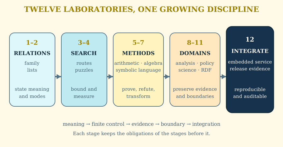
The estimates below assume familiarity with the listed chapters and include design, implementation, tests, and reflection. They are planning ranges, not deadlines.
| Laboratories | Preparation | Typical scope |
|---|---|---|
| Laboratories 1–2 | Chapters 1–5 | 2–4 hours each |
| Laboratories 3–4 | Chapters 6–10 and 13 | 4–8 hours each |
| Laboratories 5–7 | Chapters 19 and 26–29 | 4–8 hours each |
| Laboratories 8–10 | Chapters 14, 25, and 31–33 | 6–12 hours each |
| Laboratory 11 | Chapters 15–16 | 4–8 hours |
| Laboratory 12 | Chapters 16, 25, and 31–33 | multi-session capstone |
Laboratory 1. A family theory
Build: facts for at least six people and relations for parent, sibling, grandparent, and cousin.
Requirements:
- state the ground reading and principal modes of every predicate;
- expose a person being their own parent through an integrity relation;
- include one family branch that produces multiple cousins;
- query both forward and inverse modes.
Acceptance: normal output contains the predicted ground relations; one proof for a cousin conclusion passes through named intermediate concepts.
Reflect: which conclusions depend on absence, and are those closed-world assumptions justified?
Laboratory 2. A relational list toolkit
Build: user-defined relations for membership, concatenation, reversal, and prefix.
Requirements:
- use only facts, rules, unification, and list syntax for the core relations;
- document every finite mode;
- test empty, singleton, proper, and improper lists;
- compare one relation with its built-in counterpart over a finite corpus.
Acceptance: bounded differential queries find no disagreement in either direction.
Reflect: which logically meaningful modes are operationally infinite?
Laboratory 3. A cyclic transport network
Build: a network with at least ten stations, cycles, weighted edges, and two disconnected components.
Requirements:
- derive reachability;
- construct simple path witnesses;
- choose a least-cost path with deterministic tie-breaking;
- test a cycle, absence, and equal-cost routes;
- compare
--statsbefore and after one justified control improvement.
Acceptance: every returned witness begins and ends at the queried stations, uses known edges, and contains no repeated station.
Reflect: why can endpoint reachability table finitely while the set of arbitrary walks is infinite?
Laboratory 4. A finite puzzle
Build: encode a small Latin square, scheduling puzzle, or house puzzle.
Requirements:
- write the complete finite-domain calculation;
- separate generation from constraints;
- identify and remove at least one symmetry;
- retain a structured witness;
- predict the naive and symmetry-reduced search spaces.
Acceptance: the solver returns every intended solution and no permutation duplicate representing the same mathematical object.
Reflect: which source line contributes the greatest pruning power?
Laboratory 5. Arithmetic by construction
Build: Peano addition and multiplication, then one relation of your choice: exponentiation, comparison, division with remainder, or factorial.
Requirements:
- state a termination measure for each intended mode;
- prove one property by structural induction on paper;
- add a bounded executable property test;
- distinguish the inductive proof from the bounded test.
Acceptance: the proof and program share a clearly identified base and recursive structure.
Reflect: did the representation make the induction easier or merely the computation slower?
Laboratory 6. Counterexample laboratory
Build: finite operation tables over carriers of two or three elements.
Requirements:
- test closure, identity, commutativity, and associativity;
- search for a counterexample before testing the full universal property;
- return the offending tuple as a witness;
- explain which checks exhaust the model and which claims remain external.
Acceptance: one deliberately nonassociative table is rejected with a specific triple; one valid group table passes every finite law.
Reflect: why does one counterexample settle the negative question while a thousand random confirmations do not settle the positive one?
Laboratory 7. A symbolic language
Build: a small expression language with literals, variables, addition, conditionals, and local bindings.
Requirements:
- represent syntax as explicit terms;
- evaluate under an explicit environment;
- define a structural size relation;
- transform constant subexpressions;
- show that evaluation agrees before and after transformation on a finite set of environments.
Acceptance: the transformation is idempotent over the chosen corpus and does not change evaluated results.
Reflect: where is the boundary between Prolog syntax and the object language represented by Prolog terms?
Laboratory 8. A static analyzer
Build: a sign, nullness, taint, or permission analysis for a tiny statement language.
Requirements:
- define a finite abstract domain and join;
- propagate facts to a fixed point;
- emit both safe conclusions and conservative warnings;
- include a concrete execution illustrating one abstract result;
- explain the approximation direction.
Acceptance: every tested concrete behavior is covered by its abstract result; the analyzer may overapproximate but must not miss the chosen unsafe case.
Reflect: why is a warning not necessarily evidence that a concrete failure occurs?
Laboratory 9. An auditable policy
Build: an access, consent, eligibility, or compliance theory.
Requirements:
- separate source, normalized concept, decision, and reason layers;
- state every closed-world assumption;
- add at least three explicit integrity relations;
- retain source and theory version facts;
- produce proof goldens for one permit and one denial-like conclusion.
Acceptance: changing one source fact changes exactly the predicted decision and its supporting proof.
Reflect: which trust claims are established by derivation, and which require authentication outside the theory?
Laboratory 10. A scientific model
Build: encode a compact model from mechanics, circuits, chemistry, epidemiology, or statistics.
Requirements:
- document every quantity and unit;
- expose derived intermediate quantities;
- include valid, boundary, and invalid scenarios;
- use an integrity relation for an impossible input state;
- state floating-point and approximation assumptions.
Acceptance: a proof for the final classification includes measurements, equations represented by built-ins, and thresholds in an intelligible order.
Reflect: what has been proved conditionally, and what empirical claim remains outside formal logic?
Laboratory 11. An input boundary
Build: start with a small external record, validate it in JavaScript, convert it to ordinary Prolog facts, and derive one new relation.
Requirements:
- define the accepted external fields and value domains;
- keep conversion code separate from domain rules;
- query the generated Prolog program with EyeProlog directly;
- compare the final answer with a checked golden;
- document what the host authenticates.
Acceptance: invalid records are rejected before solving, valid records map to explicit finite terms, and the checked answer has an inspectable proof.
Reflect: which claims belong to host validation and which are established by the Prolog derivation?
Laboratory 12. A release-quality reasoning service
Build: combine the preceding techniques into a small embedded service.
Requirements:
- define a JavaScript boundary that supplies or loads facts;
- validate inputs before constructing the theory;
- test the principal modes and expected solution counts of public predicates;
- include semantic cases, bounded properties, metamorphic tests, integrity queries, warnings, proof goldens, and one scale case;
- retain source snapshot, theory version, and proof with every audited result;
- state time, memory, solution, and proof-size budgets;
- write a one-page trust contract and a one-page known-limitations statement.
Acceptance: another person can clone the repository, run one command, and reproduce answers and proofs from the preserved inputs without oral instructions.
Reflect: if the service gives a wrong real-world decision, which of the four trust layers—source, model, engine, or derivation—would reveal the fault?
Laboratory review rubric
Evaluate each project on five independent axes:
| Axis | Excellent work demonstrates |
|---|---|
| Meaning | every public ground relation has one stable domain sentence |
| Logic | clauses derive the intended answers and reject counterexamples |
| Control | supported modes terminate for a stated mathematical reason |
| Evidence | tests, witnesses, and proofs expose why results hold |
| Boundary | sources, assumptions, versions, limits, and host duties are named |
A beautiful program is not merely short. It makes the reason for its correctness, the shape of its search, and the boundary of its trust available to the next reader.
Historical note: logic programming grows through exercises
Logic programming has long been taught by construction. Lists, family relations, puzzles, grammars, interpreters, search problems, and small expert systems became recurring exercises because each exposes both a logical relation and the control needed to compute with it. Texts such as The Art of Prolog made this dual reading central: an exercise was not finished when a clause parsed, but when its meaning, modes, and behavior could be explained.
Laboratory practice later absorbed regression testing, property-oriented checking, benchmark corpora, and reproducible command-line runs. These tools fit logic programming unusually well because a small change can be examined at several levels at once: answers, failures, witnesses, proofs, and search. The laboratory is where a declarative claim becomes an executable experiment.
Part XI — Review
45. Checkpoint notes and selected answers
Checkpoints are for retrieval and diagnosis, not grading by hidden wording. Attempt one before reading these notes. When a checkpoint asks about a program of your own, compare the structure of your argument rather than expecting one canonical implementation.
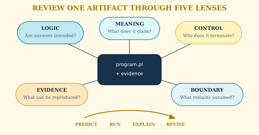
Foundations: Chapters 1–10
Chapter 1. parent(ada, byron) says that Ada is a parent of Byron.
eyeprolog --goal 'child(X, Y)' program.pl asks for every ground child–parent pair derivable by the
program. Adding parent(diego, elena). adds child(elena, diego).; it does not
change the earlier three child answers.
Chapter 2. point(X, X) unifies with point(red, red) by binding X to
red. It does not unify with point(red, blue) because one variable cannot
be both distinct atoms. [Head | Tail] unifies with [a, b, c] using
Head = a and Tail = [b, c].
Chapter 3. In
adult(Person) :- age(Person, Years), Years >= 18., a ground reading is:
every person with a recorded age of at least 18 is an adult. Operationally,
age/2 supplies Person and Years before >=/2 checks the numeric bound.
Reversing those goals asks >=/2 to inspect unbound terms.
Chapter 4. With ada → byron → clara → diego, direct ancestor answers are
the three edges. Recursive answers additionally include
ancestor(ada, clara), ancestor(byron, diego), and
ancestor(ada, diego). A successful derivation advances along a known parent
edge until a direct parent clause closes the proof.
Chapter 5. joins([a], [b, c], Whole) yields [a, b, c]. With the whole
list bound, the prefix/suffix splits are:
[]          and [a, b, c]
[a]         and [b, c]
[a, b]      and [c]
[a, b, c]   and []
[a | Tail] is not yet known to be proper because Tail might never resolve
to a finite chain ending in [].
Chapter 6. is/2, numeric comparisons, and the recursive
arithmetic steps require their documented numeric inputs. In
between(1, 10, N), an unbound N is generated from a finite interval; a
bound N is checked for membership in that interval.
Chapter 7. user(User), \+ blocked(User) first selects each known user,
then asks a ground absence question for that user.
\+ blocked(User), user(User) first asks whether the database contains no
blocked user at all. Calling either result “allowed” requires a justified,
complete user and blocked-status boundary.
Chapter 8. Over an empty nested search, findall/3 produces [],
countall/2 produces 0, and sumall/3 produces numeric zero.
aggregate_min/5 and aggregate_max/5 fail because no candidate can supply a
best key. The goal passed into the aggregate, not the aggregate’s punctuation,
must establish finiteness.
Chapter 9. message/2 is asserted as an atomic formula. Its context
argument is structured data. The program-defined context_member/2 relation
examines members inside that term; it does not add those members as globally
callable source facts.
Chapter 10. The complete coloring has six answers. Removing A \= C
leaves the requirements A ≠ B and B ≠ C, producing twelve answers. The six
new answers are those with equal first and third colors:
red–green–red, red–blue–red, green–red–green,
green–blue–green, blue–red–blue, and blue–green–blue.
Trust and construction: Chapters 11–20
Use this table to check that the checkpoint response separates concepts that are often collapsed:
| Chapter | A sound response distinguishes |
|---|---|
| 11 | ground answer, successful proof, failed search branches, and source trust |
| 12 | ordinary absence, invalid theory, process exit, and resource failure |
| 13 | structural descent, finite table growth, and unbounded term construction |
| 14 | source evidence, derived concepts, policy decisions, and integrity |
| 15 | host validation, explicit term conversion, and logical derivation |
| 16 | host validation, solver derivation, proof retention, and operational ceilings |
| 17 | ground meaning, intended mode, answer set, first answer, and proof shape |
| 18 | examples, near misses, finite generators, invariants, and presentation |
| 19 | partial correctness, completeness in a mode, and termination in that mode |
| 20 | semantic regression, observable control change, and measured improvement |
A response that says only “the program works” is incomplete. It should name the claim, the mode, the evidence inspected, and the boundary that remains outside that evidence.
Advanced work: Chapters 21–33
Later checkpoints often admit several good programs. Evaluate them with five questions:
- Meaning: is the disputed or transformed ground relation stated clearly?
- Scope: are modes, finite domains, equivalence notions, and trust assumptions explicit?
- Observation: were answers, failures, proofs, and statistics used for the different questions they can actually answer?
- Preservation: if a program changed, which semantic and observable properties were expected to remain invariant?
- Evidence: is the result reproducible as a query, test, golden output, counterexample, proof, or preserved source snapshot?
For mathematical checkpoints, add a sixth question: does the conclusion claim only what the computation warrants? One witness proves existence; one counterexample refutes a universal claim; an exhausted finite carrier proves a property only for that model; repeated bounded confirmations do not become an unbounded theorem.
For laboratory checkpoints, leave an artifact. A useful completion is not merely a paragraph: it is a small source file, predicted output, actual output, and one sentence explaining any difference.
Historical note: review becomes explanation
The declarative reading of logic programs encouraged debugging methods that ask what a relation was intended to mean, not only which machine step came next. In the early 1980s, Ehud Shapiro’s work on algorithmic debugging used computation trees together with a programmer’s judgments about intended results to narrow a fault to the clause responsible for it. Declarative debugging developed this idea alongside, rather than instead of, ordinary tracing.
That tradition gives review a distinctive role in logic programming. A worked answer is useful when it can be reconstructed from the relation, the calling mode, and the evidence, and when a disagreement can be turned into a smaller question about meaning or control. Review then becomes another pass through the same discipline as programming: predict, execute, explain, and revise.